Unreliability is the essential variable for safety functions, which are supposed to function over a certain period of time, and which cannot be maintained and repaired during this time, or only to a limited extent.
Only a few systems and their safety functions fall into this category, manned space missions, for example. What is asked here is not the frequency of failures, i. e., accidents per hour or accidents per kilometer, but the probability that the
mission will be successful, i. e. that all space travelers will return to earth in good health (hence the occasionally used term "mission time" instead of system lifetime). The mission is fixed, a simple reaching of a safe state is not possible
(although there may be abort scenarios for certain emergencies). Failures due to wear and tear during the mission can be neglected usually. All components are intensively checked before each mission so that they are like new. After launch, most
safety-related components cannot be repaired. This does not mean that there can be no diagnostics, however, this only serves to to shut down a component to prevent further damage (if this is possible) or to switch over to a replacement component
(if available).
Since few safety engineers ever have to calculate the unreliability of such systems, this chapter is kept quite short.
Of course, unreliability is not only relevant in the context of safety (rather rare there, as mentioned). Also the question "How likely is, that a new car has to go to the workshop unscheduled within the first 5 years?" is also a question about
unreliability. However, it can be answered easily without fault trees or Markov models, since there are usually no redundancies, and therefore the formulas (24) and (8) can be applied
directly, i. e.
This formula can be easily calculated using a spreadsheet even in the case of complicated time-dependent failure rates \(h_i(t)\).
7.1 Calculation with fault trees
Fault trees can be well used to calculate the unreliability of complex systems. There are two ways of calculation:
1. Directly via the unreliabilities \(F(T)\) of the basic events, using the same mathematical methods as for unavailability shown in section 5. Thus, when calculating over minimum cuts, the unreliability of each minimum cut is first calculated according to
This method is very fast, but it only works, if there are no links to unavailabilities or other probabilities which are not unreliabilities (such as the probability that an external boundary condition is satisfied). In particular, the fault tree must not
contain any conditions or INHIBIT gates. As soon as a base event describes an unavailability or other condition, this method will give too optimistic results 23.
2. Via the calculation of the failure rate \(h(t)\) (transient calculation necessary!) shown in the previous section 6 and applying the
formula (8).
The method is much slower, because the calculation of the failure rate \(h(t)\) is already more complex, and this must also be done for many points in time. However, it delivers correct results even if the failure tree contains basic events, which
describe unavailabilities or other conditions. Although this should be the exception in case of safety functions, for which the unreliability is really relevant, but may occasionally occur.
23 A good tool will warn the user accordingly or automatically switch to another algorithm
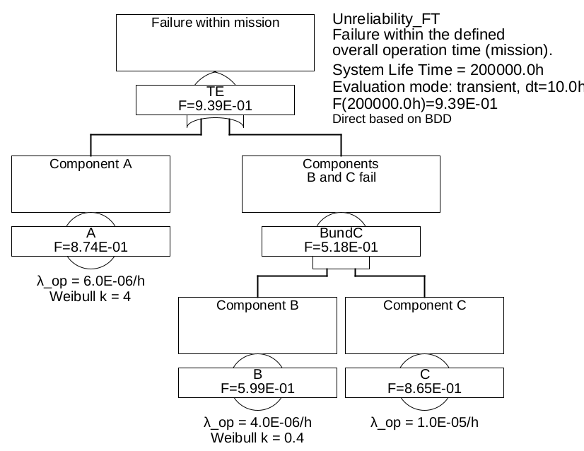
Example 7.1 For the fault tree shown in Figure 37, the
unreliability at time point \(T=\SI {200000}{\hour }\) is to be calculated using both methods presented.
Figure 37: Calculation of unreliability using fault tree
The unreliability of the basic events A and B is described here by Weibull distributions, where for A there is an increasing failure rate (Weibull exponent > 1) and for B a decreasing failure rate (Weibull exponent < 1).
Method 1:
The unreliability of the basic event A results in:
The variable order A, B, C was chosen, any other order gives the same result.
Method 2:
The failure rates of the basic events A and B are given by Formula (16), the unavailabilities \(Q(t)\) by
formula (18). The system failure rate \(h(t)\) can now be calculated with Formula (64). The unreliability is thus calculated to be \(F_{\mathrm {sys}}(T)\approx \num {0.964}\). This is somewhat too large,
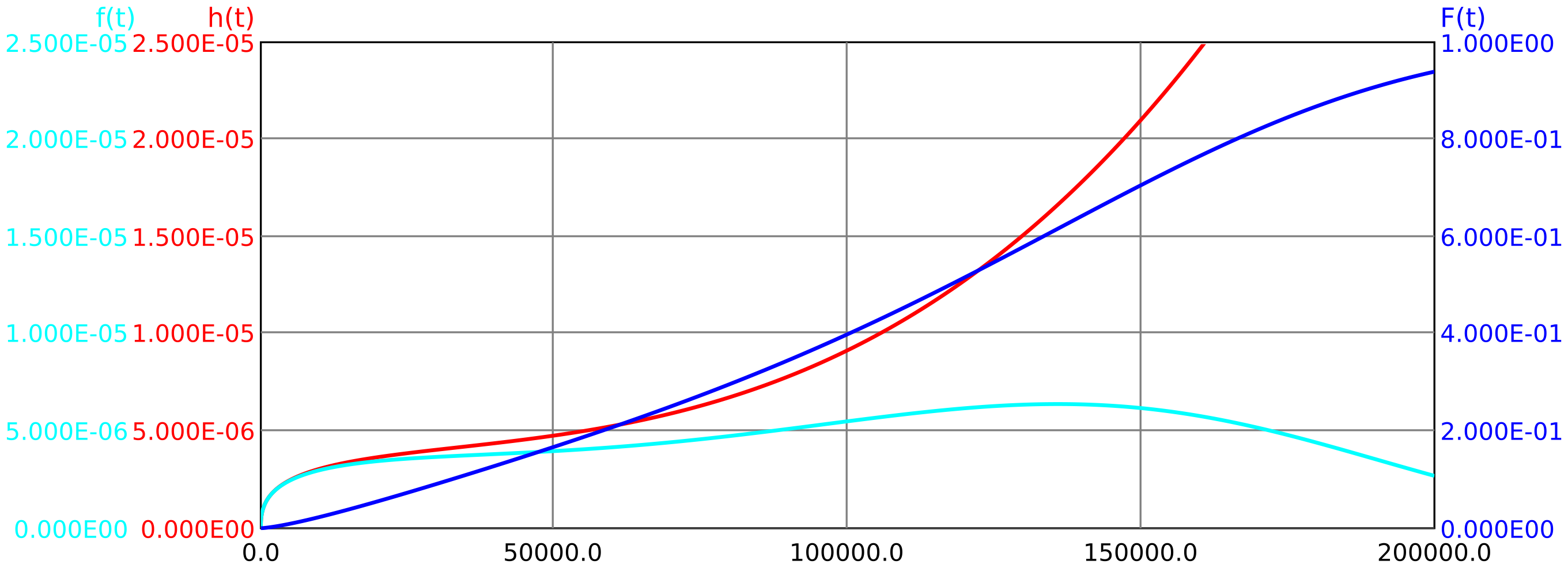
since the unavailabilities here are very large (so the system is practically unusable). If one applies instead the formula (78) from appendix B.1, the correct result is \(F_{\mathrm {sys}}(T)\approx \num {0.939}\). The time course of failure
density \(f(t)\), failure rate \(h(t)\) and unreliability \(F(t)\) is shown in Figure 38.
Figure 38: Time history of failure rate, failure density and unreliability for example 7.1
7.2 Calculation with Markov Models
The system unreliability can also be calculated using Markov models. The calculation must now basically be done by integration of the differential equation system (transient calculation), since a steady state will never be reached. The system
unreliability at a certain point in time is given by the sum of the residence probabilities in the failure states at this point in time.
If, as in example 7.1, failure distributions with non-constant failure rates are used, the transition rates are time dependent. This makes the integration
considerably more complex, since now the Jacobian matrix required for the integration of stiff differential equation systems must be inverted at least once at each time step.
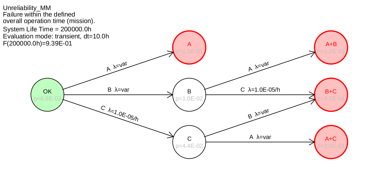
Example 7.2 Figure 39 shows the Markov model, which shows the structure of the fault
tree from example 7.1. illustrates.
Figure 39: Markov model with calculation of unreliability
The results are practically identical to those calculated in example 7.1 with fault trees.