Calculations for Functional Safety
\(\newcommand{\footnotename}{footnote}\)
\(\def \LWRfootnote {1}\)
\(\newcommand {\footnote }[2][\LWRfootnote ]{{}^{\mathrm {#1}}}\)
\(\newcommand {\footnotemark }[1][\LWRfootnote ]{{}^{\mathrm {#1}}}\)
\(\let \LWRorighspace \hspace \)
\(\renewcommand {\hspace }{\ifstar \LWRorighspace \LWRorighspace }\)
\(\newcommand {\mathnormal }[1]{{#1}}\)
\(\newcommand \ensuremath [1]{#1}\)
\(\newcommand {\LWRframebox }[2][]{\fbox {#2}} \newcommand {\framebox }[1][]{\LWRframebox } \)
\(\newcommand {\setlength }[2]{}\)
\(\newcommand {\addtolength }[2]{}\)
\(\newcommand {\setcounter }[2]{}\)
\(\newcommand {\addtocounter }[2]{}\)
\(\newcommand {\arabic }[1]{}\)
\(\newcommand {\number }[1]{}\)
\(\newcommand {\noalign }[1]{\text {#1}\notag \\}\)
\(\newcommand {\cline }[1]{}\)
\(\newcommand {\directlua }[1]{\text {(directlua)}}\)
\(\newcommand {\luatexdirectlua }[1]{\text {(directlua)}}\)
\(\newcommand {\protect }{}\)
\(\def \LWRabsorbnumber #1 {}\)
\(\def \LWRabsorbquotenumber "#1 {}\)
\(\newcommand {\LWRabsorboption }[1][]{}\)
\(\newcommand {\LWRabsorbtwooptions }[1][]{\LWRabsorboption }\)
\(\def \mathchar {\ifnextchar "\LWRabsorbquotenumber \LWRabsorbnumber }\)
\(\def \mathcode #1={\mathchar }\)
\(\let \delcode \mathcode \)
\(\let \delimiter \mathchar \)
\(\let \LWRref \ref \)
\(\renewcommand {\ref }{\ifstar \LWRref \LWRref }\)
\( \newcommand {\multicolumn }[3]{#3}\)
\(\newcommand {\toprule }[1][]{\hline }\)
\(\let \midrule \toprule \)
\(\let \bottomrule \toprule \)
\(\def \LWRbooktabscmidruleparen (#1)#2{}\)
\(\newcommand {\LWRbooktabscmidrulenoparen }[1]{}\)
\(\newcommand {\cmidrule }[1][]{\ifnextchar (\LWRbooktabscmidruleparen \LWRbooktabscmidrulenoparen }\)
\(\newcommand {\morecmidrules }{}\)
\(\newcommand {\specialrule }[3]{\hline }\)
\(\newcommand {\addlinespace }[1][]{}\)
\(\newcommand {\intertext }[1]{\text {#1}\notag \\}\)
\(\let \Hat \hat \)
\(\let \Check \check \)
\(\let \Tilde \tilde \)
\(\let \Acute \acute \)
\(\let \Grave \grave \)
\(\let \Dot \dot \)
\(\let \Ddot \ddot \)
\(\let \Breve \breve \)
\(\let \Bar \bar \)
\(\let \Vec \vec \)
\(\newcommand {\tothe }[1]{^{#1}}\)
\(\newcommand {\raiseto }[2]{{#2}^{#1}}\)
\(\newcommand {\LWRsiunitxEND }{}\)
\(\def \LWRsiunitxang #1;#2;#3;#4\LWRsiunitxEND {\ifblank {#1}{}{\num {#1}\degree }\ifblank {#2}{}{\num {#2}^{\unicode {x2032}}}\ifblank {#3}{}{\num {#3}^{\unicode {x2033}}}}\)
\(\newcommand {\ang }[2][]{\LWRsiunitxang #2;;;\LWRsiunitxEND }\)
\(\newcommand {\LWRsiunitxnumscientific }[2]{\ifblank {#1}{}{\ifstrequal {#1}{-}{-}{\LWRsiunitxprintdecimal {#1}\times }}10^{\LWRsiunitxprintdecimal {#2}} }\)
\(\def \LWRsiunitxnumplus #1+#2+#3\LWRsiunitxEND {\ifblank {#2} {\LWRsiunitxprintdecimal {#1}}{\ifblank {#1}{\LWRsiunitxprintdecimal {#2}}{\LWRsiunitxprintdecimal {#1}\unicode
{x02B}\LWRsiunitxprintdecimal {#2}}}}\)
\(\def \LWRsiunitxnumminus #1-#2-#3\LWRsiunitxEND {\ifblank {#2} {\LWRsiunitxnumplus #1+++\LWRsiunitxEND }{\LWRsiunitxprintdecimal {#1}\unicode {x02212}\LWRsiunitxprintdecimal {#2}}}\)
\(\def \LWRsiunitxnumpm #1+-#2+-#3\LWRsiunitxEND {\ifblank {#2}{\LWRsiunitxnumminus #1---\LWRsiunitxEND }{\LWRsiunitxprintdecimal {#1}\unicode {x0B1}\LWRsiunitxprintdecimal {#2}}}\)
\(\def \LWRsiunitxnumx #1x#2x#3x#4\LWRsiunitxEND {\ifblank {#2}{\LWRsiunitxnumpm #1+-+-\LWRsiunitxEND }{\ifblank {#3}{\LWRsiunitxprintdecimal {#1}\times \LWRsiunitxprintdecimal
{#2}}{\LWRsiunitxprintdecimal {#1}\times \LWRsiunitxprintdecimal {#2}\times \LWRsiunitxprintdecimal {#3}}}}\)
\(\def \LWRsiunitxnumD #1D#2D#3\LWRsiunitxEND {\ifblank {#2}{\LWRsiunitxnumx #1xxxxx\LWRsiunitxEND }{\mathrm {\LWRsiunitxnumscientific {#1}{#2}}}}\)
\(\def \LWRsiunitxnumd #1d#2d#3\LWRsiunitxEND {\ifblank {#2}{\LWRsiunitxnumD #1DDD\LWRsiunitxEND }{\mathrm {\LWRsiunitxnumscientific {#1}{#2}}}}\)
\(\def \LWRsiunitxnumE #1E#2E#3\LWRsiunitxEND {\ifblank {#2}{\LWRsiunitxnumd #1ddd\LWRsiunitxEND }{\mathrm {\LWRsiunitxnumscientific {#1}{#2}}}}\)
\(\def \LWRsiunitxnume #1e#2e#3\LWRsiunitxEND {\ifblank {#2}{\LWRsiunitxnumE #1EEE\LWRsiunitxEND }{\mathrm {\LWRsiunitxnumscientific {#1}{#2}}}}\)
\(\def \LWRsiunitxnumcomma #1,#2,#3\LWRsiunitxEND {\ifblank {#2} {\LWRsiunitxnume #1eee\LWRsiunitxEND } {\LWRsiunitxnume #1.#2eee\LWRsiunitxEND } }\)
\(\newcommand {\num }[2][]{\LWRsiunitxnumcomma #2,,,\LWRsiunitxEND }\)
\(\newcommand {\si }[2][]{\mathrm {#2}}\)
\(\def \LWRsiunitxSIopt #1[#2]#3{{#2}\num {#1}{#3}}\)
\(\newcommand {\LWRsiunitxSI }[2]{\num {#1}\,{#2}}\)
\(\newcommand {\SI }[2][]{\ifnextchar [{\LWRsiunitxSIopt {#2}}{\LWRsiunitxSI {#2}}}\)
\(\newcommand {\numlist }[2][]{\mathrm {#2}}\)
\(\newcommand {\numrange }[3][]{\num {#2}\,\unicode {x2013}\,\num {#3}}\)
\(\newcommand {\SIlist }[3][]{\mathrm {#2\,#3}}\)
\(\newcommand {\SIrange }[4][]{\num {#2}\,#4\,\unicode {x2013}\,\num {#3}\,#4}\)
\(\newcommand {\tablenum }[2][]{\mathrm {#2}}\)
\(\newcommand {\ampere }{\mathrm {A}}\)
\(\newcommand {\candela }{\mathrm {cd}}\)
\(\newcommand {\kelvin }{\mathrm {K}}\)
\(\newcommand {\kilogram }{\mathrm {kg}}\)
\(\newcommand {\metre }{\mathrm {m}}\)
\(\newcommand {\mole }{\mathrm {mol}}\)
\(\newcommand {\second }{\mathrm {s}}\)
\(\newcommand {\becquerel }{\mathrm {Bq}}\)
\(\newcommand {\degreeCelsius }{\unicode {x2103}}\)
\(\newcommand {\coulomb }{\mathrm {C}}\)
\(\newcommand {\farad }{\mathrm {F}}\)
\(\newcommand {\gray }{\mathrm {Gy}}\)
\(\newcommand {\hertz }{\mathrm {Hz}}\)
\(\newcommand {\henry }{\mathrm {H}}\)
\(\newcommand {\joule }{\mathrm {J}}\)
\(\newcommand {\katal }{\mathrm {kat}}\)
\(\newcommand {\lumen }{\mathrm {lm}}\)
\(\newcommand {\lux }{\mathrm {lx}}\)
\(\newcommand {\newton }{\mathrm {N}}\)
\(\newcommand {\ohm }{\mathrm {\Omega }}\)
\(\newcommand {\pascal }{\mathrm {Pa}}\)
\(\newcommand {\radian }{\mathrm {rad}}\)
\(\newcommand {\siemens }{\mathrm {S}}\)
\(\newcommand {\sievert }{\mathrm {Sv}}\)
\(\newcommand {\steradian }{\mathrm {sr}}\)
\(\newcommand {\tesla }{\mathrm {T}}\)
\(\newcommand {\volt }{\mathrm {V}}\)
\(\newcommand {\watt }{\mathrm {W}}\)
\(\newcommand {\weber }{\mathrm {Wb}}\)
\(\newcommand {\day }{\mathrm {d}}\)
\(\newcommand {\degree }{\mathrm {^\circ }}\)
\(\newcommand {\hectare }{\mathrm {ha}}\)
\(\newcommand {\hour }{\mathrm {h}}\)
\(\newcommand {\litre }{\mathrm {l}}\)
\(\newcommand {\liter }{\mathrm {L}}\)
\(\newcommand {\arcminute }{^\prime }\)
\(\newcommand {\minute }{\mathrm {min}}\)
\(\newcommand {\arcsecond }{^{\prime \prime }}\)
\(\newcommand {\tonne }{\mathrm {t}}\)
\(\newcommand {\astronomicalunit }{au}\)
\(\newcommand {\atomicmassunit }{u}\)
\(\newcommand {\bohr }{\mathit {a}_0}\)
\(\newcommand {\clight }{\mathit {c}_0}\)
\(\newcommand {\dalton }{\mathrm {D}_\mathrm {a}}\)
\(\newcommand {\electronmass }{\mathit {m}_{\mathrm {e}}}\)
\(\newcommand {\electronvolt }{\mathrm {eV}}\)
\(\newcommand {\elementarycharge }{\mathit {e}}\)
\(\newcommand {\hartree }{\mathit {E}_{\mathrm {h}}}\)
\(\newcommand {\planckbar }{\mathit {\unicode {x210F}}}\)
\(\newcommand {\angstrom }{\mathrm {\unicode {x212B}}}\)
\(\let \LWRorigbar \bar \)
\(\newcommand {\bar }{\mathrm {bar}}\)
\(\newcommand {\barn }{\mathrm {b}}\)
\(\newcommand {\bel }{\mathrm {B}}\)
\(\newcommand {\decibel }{\mathrm {dB}}\)
\(\newcommand {\knot }{\mathrm {kn}}\)
\(\newcommand {\mmHg }{\mathrm {mmHg}}\)
\(\newcommand {\nauticalmile }{\mathrm {M}}\)
\(\newcommand {\neper }{\mathrm {Np}}\)
\(\newcommand {\yocto }{\mathrm {y}}\)
\(\newcommand {\zepto }{\mathrm {z}}\)
\(\newcommand {\atto }{\mathrm {a}}\)
\(\newcommand {\femto }{\mathrm {f}}\)
\(\newcommand {\pico }{\mathrm {p}}\)
\(\newcommand {\nano }{\mathrm {n}}\)
\(\newcommand {\micro }{\mathrm {\unicode {x00B5}}}\)
\(\newcommand {\milli }{\mathrm {m}}\)
\(\newcommand {\centi }{\mathrm {c}}\)
\(\newcommand {\deci }{\mathrm {d}}\)
\(\newcommand {\deca }{\mathrm {da}}\)
\(\newcommand {\hecto }{\mathrm {h}}\)
\(\newcommand {\kilo }{\mathrm {k}}\)
\(\newcommand {\mega }{\mathrm {M}}\)
\(\newcommand {\giga }{\mathrm {G}}\)
\(\newcommand {\tera }{\mathrm {T}}\)
\(\newcommand {\peta }{\mathrm {P}}\)
\(\newcommand {\exa }{\mathrm {E}}\)
\(\newcommand {\zetta }{\mathrm {Z}}\)
\(\newcommand {\yotta }{\mathrm {Y}}\)
\(\newcommand {\percent }{\mathrm {\%}}\)
\(\newcommand {\meter }{\mathrm {m}}\)
\(\newcommand {\metre }{\mathrm {m}}\)
\(\newcommand {\gram }{\mathrm {g}}\)
\(\newcommand {\kg }{\kilo \gram }\)
\(\newcommand {\of }[1]{_{\mathrm {#1}}}\)
\(\newcommand {\squared }{^2}\)
\(\newcommand {\square }[1]{\mathrm {#1}^2}\)
\(\newcommand {\cubed }{^3}\)
\(\newcommand {\cubic }[1]{\mathrm {#1}^3}\)
\(\newcommand {\per }{/}\)
\(\newcommand {\celsius }{\unicode {x2103}}\)
\(\newcommand {\fg }{\femto \gram }\)
\(\newcommand {\pg }{\pico \gram }\)
\(\newcommand {\ng }{\nano \gram }\)
\(\newcommand {\ug }{\micro \gram }\)
\(\newcommand {\mg }{\milli \gram }\)
\(\newcommand {\g }{\gram }\)
\(\newcommand {\kg }{\kilo \gram }\)
\(\newcommand {\amu }{\mathrm {u}}\)
\(\newcommand {\pm }{\pico \metre }\)
\(\newcommand {\nm }{\nano \metre }\)
\(\newcommand {\um }{\micro \metre }\)
\(\newcommand {\mm }{\milli \metre }\)
\(\newcommand {\cm }{\centi \metre }\)
\(\newcommand {\dm }{\deci \metre }\)
\(\newcommand {\m }{\metre }\)
\(\newcommand {\km }{\kilo \metre }\)
\(\newcommand {\as }{\atto \second }\)
\(\newcommand {\fs }{\femto \second }\)
\(\newcommand {\ps }{\pico \second }\)
\(\newcommand {\ns }{\nano \second }\)
\(\newcommand {\us }{\micro \second }\)
\(\newcommand {\ms }{\milli \second }\)
\(\newcommand {\s }{\second }\)
\(\newcommand {\fmol }{\femto \mol }\)
\(\newcommand {\pmol }{\pico \mol }\)
\(\newcommand {\nmol }{\nano \mol }\)
\(\newcommand {\umol }{\micro \mol }\)
\(\newcommand {\mmol }{\milli \mol }\)
\(\newcommand {\mol }{\mol }\)
\(\newcommand {\kmol }{\kilo \mol }\)
\(\newcommand {\pA }{\pico \ampere }\)
\(\newcommand {\nA }{\nano \ampere }\)
\(\newcommand {\uA }{\micro \ampere }\)
\(\newcommand {\mA }{\milli \ampere }\)
\(\newcommand {\A }{\ampere }\)
\(\newcommand {\kA }{\kilo \ampere }\)
\(\newcommand {\ul }{\micro \litre }\)
\(\newcommand {\ml }{\milli \litre }\)
\(\newcommand {\l }{\litre }\)
\(\newcommand {\hl }{\hecto \litre }\)
\(\newcommand {\uL }{\micro \liter }\)
\(\newcommand {\mL }{\milli \liter }\)
\(\newcommand {\L }{\liter }\)
\(\newcommand {\hL }{\hecto \liter }\)
\(\newcommand {\mHz }{\milli \hertz }\)
\(\newcommand {\Hz }{\hertz }\)
\(\newcommand {\kHz }{\kilo \hertz }\)
\(\newcommand {\MHz }{\mega \hertz }\)
\(\newcommand {\GHz }{\giga \hertz }\)
\(\newcommand {\THz }{\tera \hertz }\)
\(\newcommand {\mN }{\milli \newton }\)
\(\newcommand {\N }{\newton }\)
\(\newcommand {\kN }{\kilo \newton }\)
\(\newcommand {\MN }{\mega \newton }\)
\(\newcommand {\Pa }{\pascal }\)
\(\newcommand {\kPa }{\kilo \pascal }\)
\(\newcommand {\MPa }{\mega \pascal }\)
\(\newcommand {\GPa }{\giga \pascal }\)
\(\newcommand {\mohm }{\milli \ohm }\)
\(\newcommand {\kohm }{\kilo \ohm }\)
\(\newcommand {\Mohm }{\mega \ohm }\)
\(\newcommand {\pV }{\pico \volt }\)
\(\newcommand {\nV }{\nano \volt }\)
\(\newcommand {\uV }{\micro \volt }\)
\(\newcommand {\mV }{\milli \volt }\)
\(\newcommand {\V }{\volt }\)
\(\newcommand {\kV }{\kilo \volt }\)
\(\newcommand {\W }{\watt }\)
\(\newcommand {\uW }{\micro \watt }\)
\(\newcommand {\mW }{\milli \watt }\)
\(\newcommand {\kW }{\kilo \watt }\)
\(\newcommand {\MW }{\mega \watt }\)
\(\newcommand {\GW }{\giga \watt }\)
\(\newcommand {\J }{\joule }\)
\(\newcommand {\uJ }{\micro \joule }\)
\(\newcommand {\mJ }{\milli \joule }\)
\(\newcommand {\kJ }{\kilo \joule }\)
\(\newcommand {\eV }{\electronvolt }\)
\(\newcommand {\meV }{\milli \electronvolt }\)
\(\newcommand {\keV }{\kilo \electronvolt }\)
\(\newcommand {\MeV }{\mega \electronvolt }\)
\(\newcommand {\GeV }{\giga \electronvolt }\)
\(\newcommand {\TeV }{\tera \electronvolt }\)
\(\newcommand {\kWh }{\kilo \watt \hour }\)
\(\newcommand {\F }{\farad }\)
\(\newcommand {\fF }{\femto \farad }\)
\(\newcommand {\pF }{\pico \farad }\)
\(\newcommand {\K }{\mathrm {K}}\)
\(\newcommand {\dB }{\mathrm {dB}}\)
\(\newcommand {\kibi }{\mathrm {Ki}}\)
\(\newcommand {\mebi }{\mathrm {Mi}}\)
\(\newcommand {\gibi }{\mathrm {Gi}}\)
\(\newcommand {\tebi }{\mathrm {Ti}}\)
\(\newcommand {\pebi }{\mathrm {Pi}}\)
\(\newcommand {\exbi }{\mathrm {Ei}}\)
\(\newcommand {\zebi }{\mathrm {Zi}}\)
\(\newcommand {\yobi }{\mathrm {Yi}}\)
\(\newcommand {\LWRsubmultirow }[2][]{#2}\)
\(\newcommand {\LWRmultirow }[2][]{\LWRsubmultirow }\)
\(\newcommand {\multirow }[2][]{\LWRmultirow }\)
\(\newcommand {\mrowcell }{}\)
\(\newcommand {\mcolrowcell }{}\)
\(\newcommand {\STneed }[1]{}\)
\(\def \LWRsiunitxprintdecimalsub #1,#2,#3\LWRsiunitxEND {\mathrm {#1}\ifblank {#2}{}{.\mathrm {#2}}}\)
\(\newcommand {\LWRsiunitxprintdecimal }[1]{\LWRsiunitxprintdecimalsub #1,,,\LWRsiunitxEND }\)
C Other distribution functionsC.1 Normal distribution
The normal distribution (Gaussian distribution) has the density function
\(\seteqnumber{0}{}{78}\)
\begin{equation}
f(t)=\frac {1}{\sqrt {2\pi \sigma ^2}}\,\mathrm {e}^{-\,\dfrac {(t-\mu )^2}{2\sigma ^2}}
\end{equation}
with the mean \(\mu =\mathrm {MTTF}\) and the standard deviation \(\sigma \). It should be noted, that the function already starts at \(t=-\infty \) and that this proportion cannot be set to 0.
Consequently, the distribution function is given by
\(\seteqnumber{0}{}{79}\)
\begin{equation}
F(t)=\int \limits _{-\infty }^x f(t) dt = \frac {1}{\sqrt {2\pi \sigma ^2}} \int \limits _{-\infty }^x \mathrm {e}^{-\,\dfrac {(t-\mu )^2}{2\sigma ^2}} dt =\num {0.5}\left (1+\mathrm
{erf}\left (\dfrac {t-\mu }{\sqrt {2\sigma ^2}} \right )\right )
\end{equation}
where \(\mathrm {erf(x)}\) is the so-called error function. There is no closed representation for this integral, it must therefore always be determined numerically. Accordingly, there is also no closed representation for the failure rate \(h(t)\).
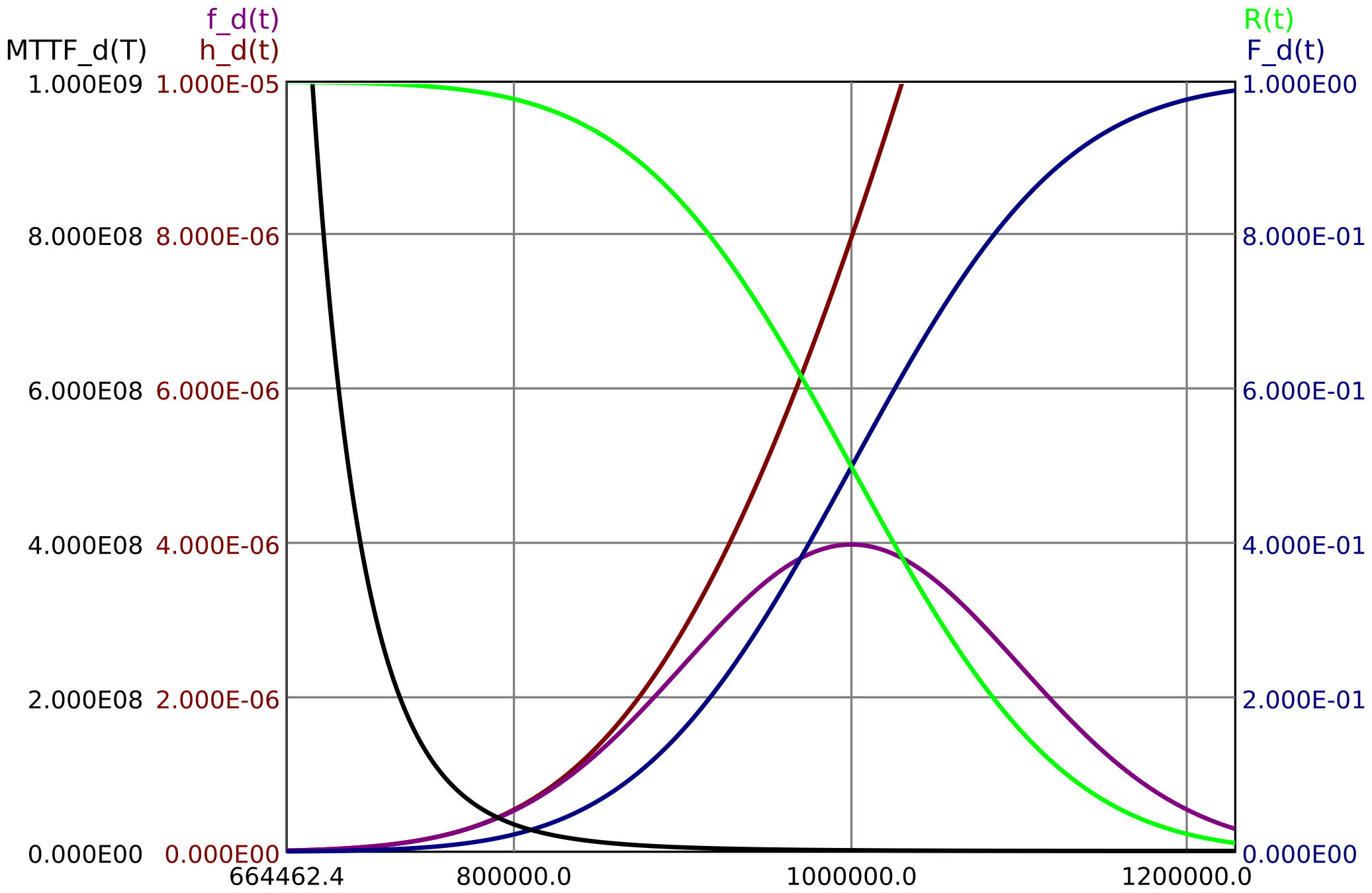
The figure 40 shows a normal distribution with mean \(\mu =\SI {1e6}{\hour }\) and standard deviation \(\sigma =\SI {1e5}{\hour }\).
Figure 40: Normal distribution with mean \(\mu =\SI {1e6}{\hour }\) and standard deviation \(\sigma =\SI {1e5}{\hour }\)
C.2 Uniform distribution
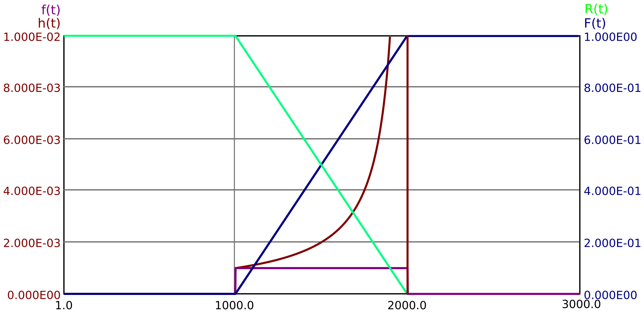
The uniform distribution is characterized by a constant outage density \(f(t)=\mathrm {const}\) within an interval \(t_1 \dots t_2\). Outside this interval it is 0. It is therefore also called a rectangular distribution. It does not occur in
nature and technology, but it is suitable for thought experiments or for plausibility checks of formulas.
\(\seteqnumber{0}{}{80}\)
\begin{equation}
f(t)=\dfrac {1}{t_2 - t_1} \quad \text {for } t_1 \leq t < t_2 \quad \text {, else 0}
\end{equation}
\(\seteqnumber{0}{}{81}\)
\begin{equation}
F(t)=\begin{cases} 0 & \text {for } t<t_1 \\ \dfrac {t-t_1}{t_2-t_1} & \text {for } t_1 \leq t < t_2 \\ 1 & \text {for } t \geq t_2 \end {cases}
\end{equation}
\(\seteqnumber{0}{}{82}\)
\begin{equation}
R(t)=\begin{cases} 1 & \text {for } t<t_1 \\ \dfrac {t_2-t}{t_2-t_1} & \text {for } t_1 \leq t < t_2 \\ 0 & \text {for } t \geq t_2 \end {cases}
\end{equation}
\(\seteqnumber{0}{}{83}\)
\begin{equation}
h(t)=\dfrac {\,\frac {1}{t_2-t_1}\,}{\frac {t_2-t}{t_2-t_1}} =\frac {1}{t_2-t_1} \cdot \frac {t_2-t_1}{t_2-t} =\frac {1}{t_2-t} \quad \text {for } t_1 \leq t < t_2 \quad \text {, else
0}
\end{equation}
\(\seteqnumber{0}{}{84}\)
\begin{equation}
\mathrm {MTTF}=\int \limits _{t_1}^{t_2} t \cdot \frac {1}{t_2 - t_1} \,dt = \frac {1}{t_2-t_1} \left [ \frac {t^2}{2} \right ]_{t_1}^{t_2} \\ = \frac {1}{t_2-t_1} \, \frac
{t_2^2-t_1^2}{2} = \frac {t_1+t_2}{2}
\end{equation}
A uniform distribution is shown in Figure 41 . It can be seen that the failure rate \(h(t)\) approaches infinity for \(t \rightarrow t_2\),
i. e., has a pole at \(t_2\).
Figure 41: Uniform distribution between \(t_1\) and \(t_2\)
C.3 Dirac distribution
The Dirac distribution is the mathematical description of determinism: Only at time \(T\) does the density \(f(t)\) take a value other than 0. Thus, the density must have the property of a Dirac shock of height 1 at time \(T\):
\(\seteqnumber{0}{}{85}\)
\begin{equation}
f(t)=\delta (t-T)
\end{equation}
Here \(\delta (t)\) is the Dirac function with the property \(\int _{-\infty }^{+\infty }\delta (t)\,dt=1\). So at time \(T\) the unreliability jumps from 0 to 1:
\(\seteqnumber{0}{}{86}\)
\begin{equation}
F(t)=\int \limits _{0}^{\infty } f(t)\,dt =\int \limits _{0}^{\infty } \delta (t-T)\,dt =\sigma (t-T)
\end{equation}
Here \(\sigma (t-T)\) denotes the unit jump function at time \(T\). For the reliability, the immediate result is:
\(\seteqnumber{0}{}{87}\)
\begin{equation}
R(t)=1-\sigma (t-T)
\end{equation}
The MTTF is obviously \(T\), which also results computationally:
\(\seteqnumber{0}{}{88}\)
\begin{equation}
\mathrm {MTTF}=\int \limits _{0}^{\infty } t \cdot \delta (t-T) \,dt = T
\end{equation}
The delta distribution is a special case of numerous distributions, for example the uniform distribution (namely for \(t_1 \rightarrow t_2\)) or the normal distribution (for scatter \(\sigma \rightarrow 0\)).