Calculations for Functional Safety
Quantities, Formulas and Methods

2 Reliability and related variables

2.1 Reliability and unreliability

Reliability \(R(t_1,t_2)\) is the probability, that a component/system/function does not fail in the time interval \(t_1\) to \(t_2\), regardless of whether it was working at time \(t_1\).

Unreliability \(F(t_1,t_2)\) is the probability, that a component/system/function fails in the time interval \(t_1\) to \(t_2\), regardless of whether it was working at time \(t_1\). Consequently, it is the complementary probability (or converse probability) to the reliability:

\begin{equation} F(t_1,t_2) = 1 - R(t_1,t_2) \quad \textrm {or} \quad R(t_1,t_2) = 1 - F(t_1,t_2) \end{equation}

For practically all questions one chooses \(t_1=0\) and thus obtains the one-parameter functions \(R(t_1=0,t_2=t)=R(t)\) and \(F(t_1=0,t_2=t)=F(t)\). For the relationship between reliability and unreliability, the following applies accordingly:

\begin{equation} F(t) = 1 - R(t) \quad \textrm {or} \quad R(t) = 1 - F(t) \end{equation}

\(F(t)\) is sometimes also referred to as the probability of survival.

Note: Unreliability is often called probability of failure. However, unavailability is also often called probability of failure, although it is a completely different quantity. To avoid misunderstandings, the term "probability of failure" should not be used, therefore.

Note: Especially for vehicles, one sometimes relates reliability and also subsequent quantities to the distance \(s\) traveled. \(F(t_1,t_2)\) then becomes \(F(s_1,s_2)\) etc. In all formulas given, the time must then be replaced by the distance.

Example 2.1 Let the probability \(p\) be asked, that a component with age \(t\) will fail within the next hour. It should not be assumed that it is still working at time \(t\):
\(\seteqnumber{0}{}{2}\)
\begin{equation*} p=F(t,t+1\,\mathrm {h})=F(t+1\,\mathrm {h})-F(t) \end{equation*}

Example 2.2 Let the probability \(p\) be asked, that a component with age \(t\), which is still working at time \(t\) will fail within the next hour:
\(\seteqnumber{0}{}{2}\)
\begin{equation*} p=\frac {F(t,t+1\,\mathrm {h})}{R(t)}=\frac {F(t+1\,\mathrm {h})-F(t)}{R(t)} =\frac {R(t)-R(t+1\,\mathrm {h})}{R(t)} \end{equation*}

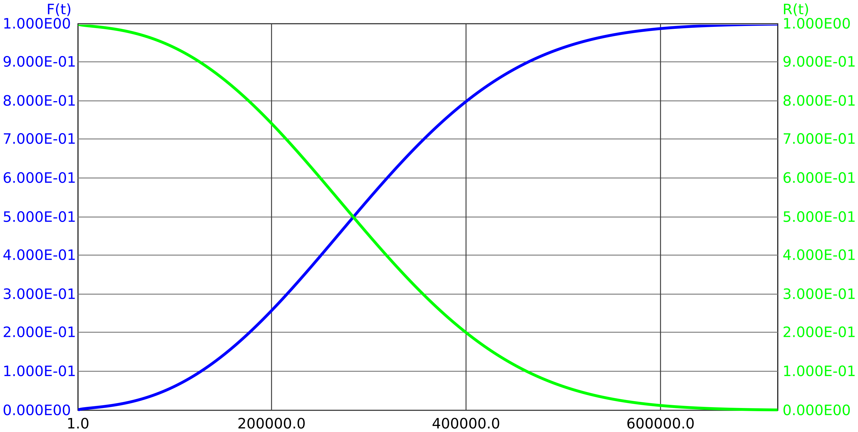
Example 2.3 It is known from many years of experience, that the reliability and unreliability follows the (cumulative) distribution functions shown in Figure 1.

Figure 1: Example reliability and unreliability function

Question 1: What is the probability that the component will work for more than 40.000 hours?

Answer: \(p=R(\SI {40000}{\hour }) \approx \num {0.2}\). Consequently, the component will work longer than 40000 hours with 20% probability.

Question 2: What is the probability, that the component will fail between 40000 and 50000 operating hours?

Answer: \(p=F(\SI {50000}{\hour })-F(\SI {40000}{\hour })=R(\SI {40000}{\hour })-R(\SI {50000}{\hour })\approx \num {0.15}\). So the component will fail with 15% probability after 40000 to 50000 hours.

Question 3: What is the probability that the component will fail between 40000 and 50000 hours of operation, if it was still working at 40000 hours?

Answer: \(p=\dfrac {F(\SI {50000}{\hour })-F(\SI {40000}{\hour })}{R(\SI {40000}{\hour })}\approx \dfrac {\num {0.15}}{\num {0.2}}=\num {0.75}\).

2.2 Failure density and failure rate

The change in unreliability per time is the failure density. For any failure density function \(f(t)\) holds:

\begin{equation} F(t) = \int \limits _0^t f(\tau )\;d\tau \quad \textrm {or} \quad f(t) = \frac {dF(t)}{dt} = -\,\frac {dR(t)}{dt} \end{equation}

Unlike unreliability, failure density is not a probability. It can take any positive value and has a dimension (usually 1/time or 1/distance).

Since the unreliability for \(t \rightarrow \infty \) approaches 1, the following must hold for any density function:

\begin{equation} \int \limits _0^\infty f(\tau )\;d\tau = 1 \end{equation}

The failure rate \(h(t)\) for arbitrary failure density functions is given as

\begin{equation} h(t) = \frac {f(t)}{R(t)} = \frac {f(t)}{1-F(t)} \end{equation}

With \(f(t) = -\frac {dR(t)}{dt}\) we get:

\begin{equation} h(t) = \frac {f(t)}{R(t)} = \frac {-dR(t)/dt}{R(t)} = -\,\frac {\dot {R}}{R} \end{equation}

\begin{equation} R(t) = \mathrm {e}^{-\int \limits _0^t h(\tau )\,d\tau } \end{equation}

\begin{equation} \label {eq:F_h} F(t) = 1-\mathrm {e}^{-\int \limits _0^t h(\tau )\,d\tau } \end{equation}

A failure distribution is fully described by \(f(t)\) or \(F(t)\) or \(R(t)\) or \(h(t)\)

Figure 2 shows an example failure distribution and the quantities describing it.

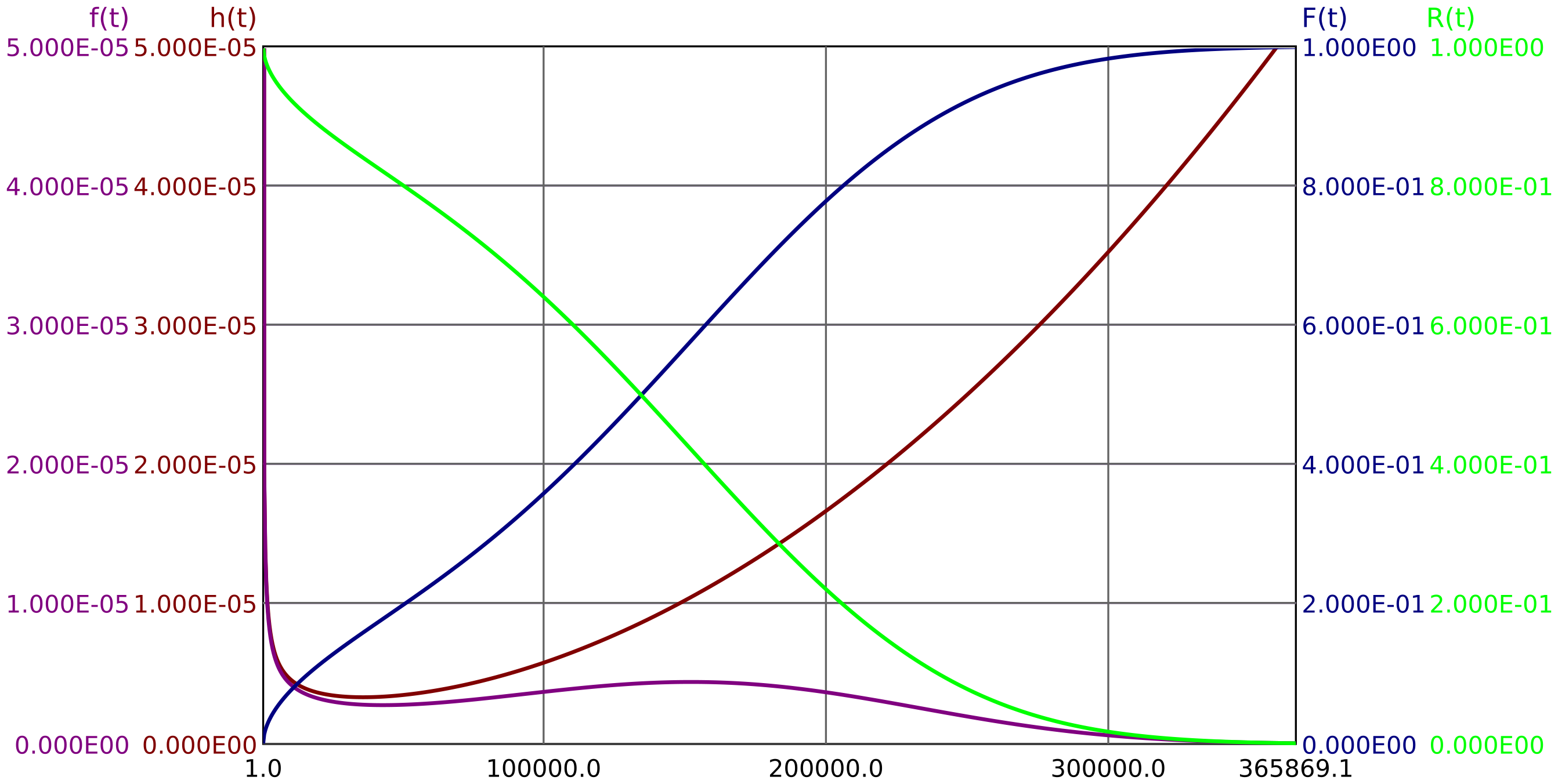
Note: While the symbols \(R(t)\), \(F(t)\) and also \(f(t)\) are largely uniformly used, no symbol has yet been established for the failure rate. Instead of \(h(t)\) one also finds \(\Lambda (t)\) or \(\lambda (t)\).

The failure rate \(h(t)\) indicates the probability of a failure per time interval, under the condition that the function has not failed at the beginning of the time interval:

\begin{equation} h(t) = \frac {f(t)}{R(t)} = \frac {dF(t)/dt}{R(t)} = \frac {1}{R(t)}\,\lim _{\Delta t \rightarrow 0} \frac {F(t+\Delta t) - F(t)}{\Delta t} \end{equation}

Here the time interval \(\Delta t\) must be sufficiently small! Therefore this equation must not be used to calculate an average failure rate over a longer period of time. The formulas required for this purpose are mentioned in section 3.

2.3 Bathtub curve

Each non-trivial component can fail in different ways. Each of these failure modes has its own failure distribution function. There are almost always failure modes with decreasing failure rate, these are usually due to production defects. For mechanical or even heavily loaded electronic components, there are also failure modes with increasing failure rate, these are in particular the failures due to wear or aging. The total failure rate is obtained by adding the individual failure rates of all n failure modes:

\begin{equation} h(t) = \sum _{i=1}^n h_i(t) \end{equation}

As soon as there is at least one failure mode with falling failure rate and one with rising failure rate, the graph of the total failure rate \(h(t)\) resembles a bathtub, see figure 2.

2.4 Mean Time to Failure (MTTF)

The Mean Time To Failure (MTTF) is the expected value of the time until failure. It is calculated for any failure distribution as follows:

\begin{equation} \label {eq:MTTF} \mathrm {MTTF} = \int \limits _0^\infty t \cdot f(t)\,dt \end{equation}

This value is referred to as natural MTTF in section 3, since it is the (arithmetic) mean value which is obtained experimentally, if the component is always operated until failure and then replaced. In practice, however, this is often not the case, so that other formulas apply, especially for the determination of mean failure rates, see section 3.

2.5 Distribution functions

In this section, some distribution functions are presented, which are relevant in practice or for subsequent considerations. Further distributions are described in Appendix C.

2.5.1 Exponential distribution

The exponential distribution is characterized by a constant failure rate \(h(t)=const\). The failure rate is therefore described by a single parameter, which is denoted by \(\lambda \). The exponential distribution is the simplest and at the same time most important distribution function. It is true for memoryless components, i. e. when the age of the component has no significant influence on the failure rate (also called ergodic behavior). The time course of reliability \(R(t)\), unreliability \(F(t)\), failure rate \(h(t)\) and failure density \(f(t)\) is shown in Figure 3.

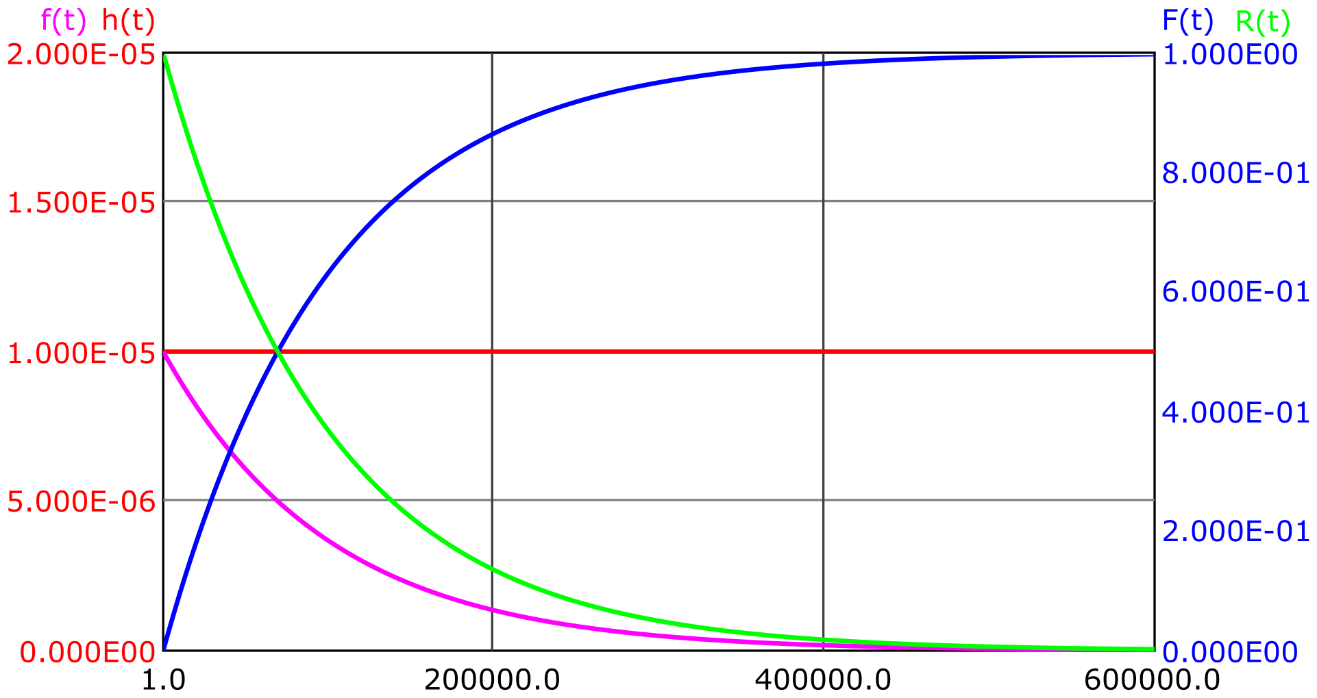
The exponential distribution is described by the following equations:

\begin{equation} f(t)=\lambda \cdot \mathrm {e}^{-\lambda \cdot t} \end{equation}

\begin{equation} F(t) = 1 - \mathrm {e}^{-\lambda \cdot t} \end{equation}

\begin{equation} R(t) = \mathrm {e}^{-\lambda \cdot t} \end{equation}

The mean time to failure is:

\begin{equation} \mathrm {MTTF} = \int _0^\infty t \cdot \lambda \cdot \mathrm {e}^{-\lambda \cdot t}\,dt = - \frac { \left ( \lambda \cdot t + 1 \right ) \, \mathrm {e}^{-\lambda \cdot t} } {\lambda } \Big |_0^\infty = \frac {1}{\lambda } \end{equation}

Example 2.4 What is the probability \(p\), that a component with age \(t\), which is still working at time \(t\), will fail within the next hour. Let it be known that the component can be described by a constant failure rate.
\(\seteqnumber{0}{}{15}\)
\begin{align*} p=\frac {F(t,t+1\,\mathrm {h})}{R(t)} &=\frac {F(t+1\,\mathrm {h})-F(t)}{R(t)} = \frac {\mathrm {e}^{-\lambda \cdot t} - \mathrm {e}^{-\lambda \cdot (t+1\,\mathrm {h})}} {\mathrm {e}^{-\lambda \cdot t}} \\ &= \frac {\mathrm {e}^{-\lambda \cdot t} - \mathrm {e}^{-\lambda \cdot t} \cdot \mathrm {e}^{-\lambda \cdot 1\,\mathrm {h}}} {\mathrm {e}^{-\lambda \cdot t}} = 1 - \mathrm {e}^{-\lambda \cdot 1\,\mathrm {h}} \end{align*} As expected, the age of the component \(t\) does not appear in the result.

Many elements can be described with sufficient accuracy by a constant failure rate. In particular, for elements of a system whose MTTF is much shorter than the overall system service life (and will therefore be replaced multiple times after failure, e. g. a conventional light bulb in a lamp), and which are not replaced preventively at certain pre-defined points in time, only a constant mean failure rate \(h(t)=\overline {h}=\lambda \) can be specified within the scope of system calculations, since the actual failure rate function itself is random.

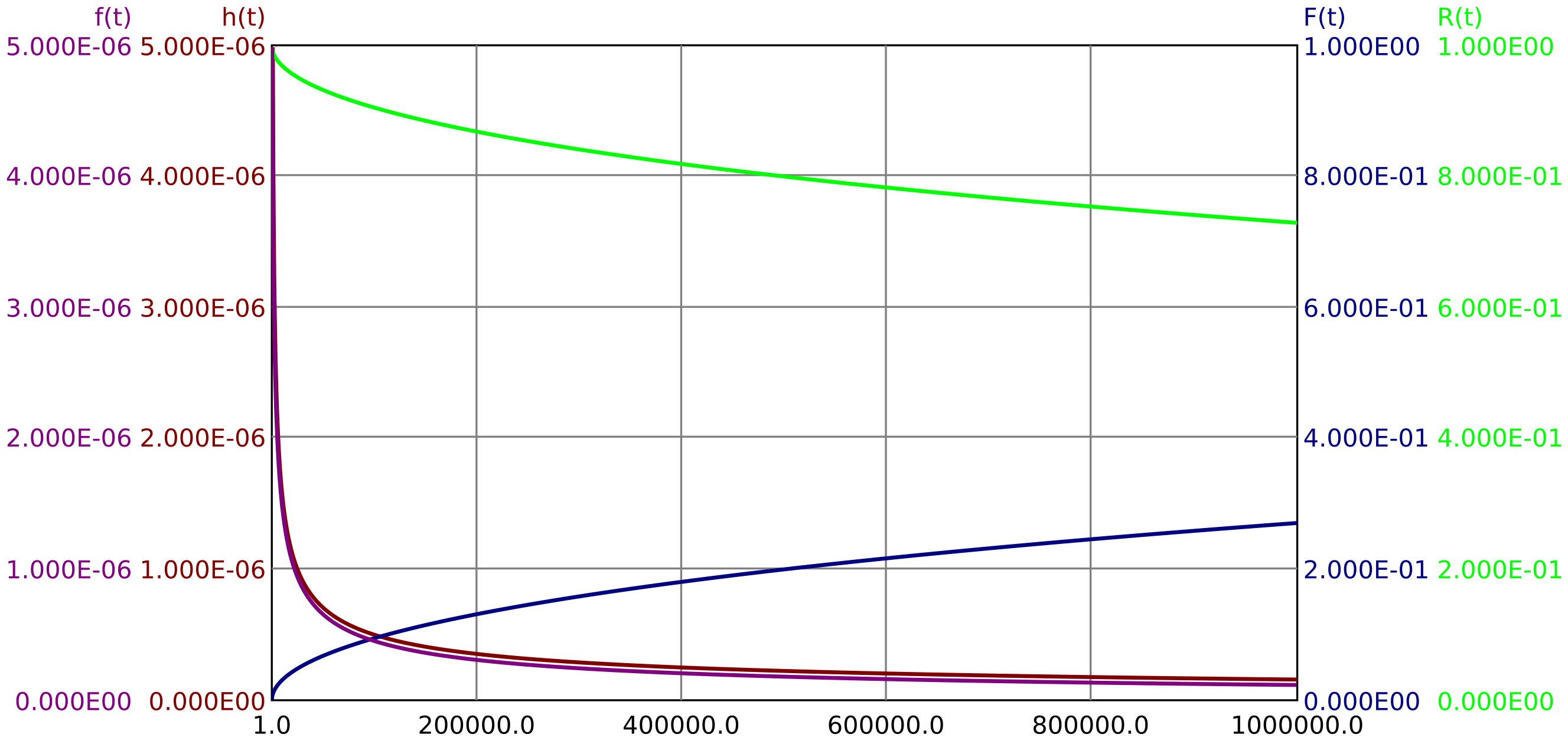
2.5.2 Weibull distribution

The Weibull distribution is a generalization of the exponential distribution. With an additional parameter \(k>0\) in the exponent, falling or rising default rates can be modeled. For \(0<k<1\) a falling, for \(k>1\) an increasing failure rate results. For \(k=1\) the result is the exponential distribution.

\begin{equation} \label {eq:Weibull_h} h(t) = \lambda \cdot k \cdot (\lambda \cdot t)^{k-1} \end{equation}

\begin{equation} \label {eq:Weibull_f} f(t)=\lambda \cdot k \cdot (\lambda \cdot t)^{k-1} \mathrm {e}^{-(\lambda \cdot t)^k} \end{equation}

\begin{equation} \label {eq:Weibull_F} F(t) = 1 - \mathrm {e}^{-(\lambda \cdot t)^k} \end{equation}

\begin{equation} \mathrm {MTTF} = \frac {1}{\lambda } \cdot \Gamma \left (1+\frac {1}{k}\right ) \end{equation}

Failure modes that are exclusively due to wear and tear, can usually be completely excluded for a certain time \(t_0\). These failure modes can usually be well modeled with a Weibull distribution with \(k>1\) (increasing failure rate), which is additionally shifted to the right by \(t_0>0\):

\begin{equation} h(t) = \lambda \cdot k \cdot (\lambda \cdot (t-t_0))^{k-1} \quad \text {for}~t>t_0 \end{equation}

Note: Especially in English-speaking countries, the Weibull distribution is often parameterized with \(\mu =1/\lambda \).

Figures 4 and 5 show a Weibull distribution with decreasing failure rate (k=0.5) and with increasing failure rate (k=3).

2.5.3 Mortality

Human mortality is also a distribution function, although it does not directly follow a mathematical function. Figure 6 shows a cross-sectional view of the mortality of the mortality of the West German population in the years 1960-1962 is shown.

The cross-sectional analysis is based on the statistics of deaths during the period in question. It thus makes a statement in particular about the actual mean age at death of the people who died in this period. The mortality rate \(h(t)\) thus indicates the probability here, that a person who had reached the age \(t\) dies within the time span \(\Delta t\), divided by this time span \(\Delta t\).

In contrast to the cross-sectional view, the so-called longitudinal view makes a statement about the mortality distribution of the people born in the respective period. Longitudinal statistical observations can therefore only be made for birth cohorts, of which no human being is still alive. For later cohorts, they represent forecasts in whole or in part. If the mortality distribution were independent of the year of birth, the cross-sectional and longitudinal distributions would be identical. For the longitudinal view, the quantities are immediately illustrative:

• Reliability (survival probability) \(R(t)\) is the probability of reaching age \(t\).
• The unreliability (failure probability) \(F(t)\) is the probability of dying before reaching age \(t\).
• The failure density \(f(t)\) is the probability of dying at age between \(t\) and \(t+\Delta t\), divided by the period \(\Delta t\), with \(\Delta t \rightarrow 0\).
• The failure rate \(h(t)\) is the probability of dying at age between \(t\) and \(t+\delta t\), given the condition of having reached age \(t\), divided by the period \(\Delta t\), with \(\Delta t \rightarrow 0\).
• The MTTF is the life expectancy of a newborn.

Calculations for Functional Safety Quantities, Formulas and Methods