Calculations for Functional Safety
Quantities, Formulas and Methods
3 Mean failure rate and mean time to failure
For many components, the failure rate is highly time dependent. A mean failure rate is also often required for such components, among others for the following reasons:
-
• If system variables (\(\overline {h_{\mathrm {sys}}}\), \(\overline {Q_{\mathrm {sys}}}\)) are to be calculated in a stationary way, only mean failure rates can be used due to the principle.
-
• If a component is likely to fail (and be replaced or repaired) multiple times during the system’s operational lifetime, from the first failure on, the failure rate function itself is also a random variable, which becomes increasingly fuzzy as the number of failures (and thus replacements) increases. Even in the case of transient, i. e. continuously time-resolved, observations, no failure rate function can be given.
-
• If the component is to be replaced regularly as a preventive measure, so that it will most probably not fail, the question arises at what interval the component should be replaced, in order to keep the effective (residual) failure rate and thus the probability of failure as low as possible.
Therefore, in this section, the following tasks will be addressed:
-
1. What are the MTTF and mean failure rate for the case, that the component is operated until failure and then replaced? (Example: light bulb)
-
2. What are MTTF and effective mean failure rate for the case, that the component is regularly replaced as a preventive measure? (Example: timing belt of a car combustion engine)
-
3. If there are dangerous and non-dangerous failure modes of a component: How can the dangerous MTTF and dangerous mean failure rate be calculated for the above two cases?
It is often claimed, one should use the failure rate in the flat area of the "bathtub curve" for such questions. However, this is only correct if the component is really only operated in this range, i. e. early failures (especially production defects) can be absolutely excluded as well as failures due to aging and wear. These conditions are very often not met – and moreover, the bathtub curve often does not show a really flat area at all. Instead, so-called early failures overlap with late failures.
Note: Some readers may wonder, why the abbreviation MTTF is also used for the time between two failures, and not MTBF (Mean Time Between Failures). The answer is simple, that almost always when MTBF is mentioned, actually the MTTF is meant (or necessary in fact). In applications or calculations, where fault detection times or repair times are not insignificant, these must be explicitly mentioned anyway. Thus, there is no valid reason, neither in safety nor in reliability theory, to introduce or use a quantity "MTBF". 2
2 In fact, I am not sure, if I have ever seen a document in which the term MTBF has been used correctly – apart from theoretical textbooks
3.1 MTTF in long use without preventive replacement
First, the MTTF and the mean failure rate are to be calculated for a component, which has a significantly lower life expectancy than the nominal service life of the overall system. In this case, it can be assumed that the component will fail several times and will therefore have to be replaced several times.
For arbitrary failure distribution functions, the following holds:
\(\seteqnumber{0}{}{20}\)\begin{equation} \label {eq:MTTF_int_tf} \mathrm {MTTF} = \int \limits _0^\infty t \cdot f(t)\, dt \end{equation}
If sufficient test or field data is available, then this integral can be easily calculated with a spreadsheet. If instead of \(f(t)\) the data \(F(t)\) or \(R(t)\) are available, \(f(t)\) can be easily obtained by numerical differentiation.
In general, the following applies to the failure density function
\(\seteqnumber{0}{}{21}\)\begin{equation} f(t) = h(t) \cdot R(t) = h(t) \cdot \mathrm {e}^{-\int \limits _0^t h(\tau )\,d\tau } \end{equation}
and thus for the MTTF
\(\seteqnumber{0}{}{22}\)\begin{equation} \mathrm {MTTF} = \int \limits _0^\infty t \cdot h(t) \cdot \mathrm {e}^{-\int \limits _0^t h(\tau )\,d\tau }\;dt \end{equation}
Almost all components have multiple failure modes, which obey different failure distribution functions. Assuming that the failure distribution functions of the individual failure modes are known, how can the MTTF be calculated? For this, it must be assumed that the failure modes are independent of each other, i. e. they do not influence each other. In order for this prerequisite to be fulfilled it is necessary in particular that the component is replaced in the case of each failure. Then it holds for the total failure rate function \(h(t)\) of the component, that it is given by the sum of the failure rate functions of the individual failure modes:
\(\seteqnumber{0}{}{23}\)\begin{equation} \label {eq:h_sum} h(t) = \sum _{i=1}^n h_i(t) \end{equation}
If both all \(h_i(t)\) and the respective associated reliability functions \(R_i(t)\) are given by mathematical formulas, it is helpful to simplify the double integral:
\(\seteqnumber{0}{}{24}\)\begin{align} \label {eq:MTTF_vollstaendig} \begin{split} \mathrm {MTTF} &= \int \limits _0^\infty t \cdot h(t) \cdot \mathrm {e}^{-\int \limits _0^t \sum \limits _{i=1}^n h_i(\tau )\,d\tau }\;dt = \int \limits _0^\infty t \cdot h(t) \cdot \mathrm {e}^{-\sum \limits _{i=1}^n \int \limits _0^t h_i(\tau )\,d\tau }\;dt\\ &= \int \limits _0^\infty t \cdot h(t) \cdot \prod _{i=1}^n R_i(t)\;dt \end {split} \end{align} The MTTF determined in this way is called complete MTTF or natural MTTF, because it is the mean time to failure that results, if the component is used until failure and then replaced (as is the case in long-life systems such as machinery, aircraft, or rail vehicles).
The average failure rate of the component in the event, that the component is likely to fail (several times) and is then replaced each time, is the reciprocal of the complete MTTF:
\(\seteqnumber{0}{}{25}\)\begin{equation} \label {eq:lambda_MTTF} \lambda = \frac {1}{\mathrm {MTTF}} \end{equation}
3.2 Preventive Exchange and Incomplete MTTF
In the case of preventive replacement after a time interval \(T\), the incomplete MTTF(T) is required for the time interval 0 to \(T\). The same applies if the natural MTTF of the component is much greater than the lifetime of the system in which it is used. From considerations which cannot be reproduced here, it follows:
\(\seteqnumber{0}{}{26}\)\begin{equation} \mathrm {MTTF}(T) = \frac {\int \limits _0^T t\cdot f(t)\,dt +T\cdot R(T)}{F(T)} \end{equation}
With \(R(T)=1-F(T)\) and the already known formulas for the relationship between reliability and failure rate, one obtains a formula for calculating \(\mathrm {MTTF}(T)\) for a given or experimentally determined failure rate function \(h(t)\):
\(\seteqnumber{0}{}{27}\)\begin{align} \label {eq:mttf_T} \begin{split} \mathrm {MTTF(T)} &= \frac {\int \limits _0^T t\cdot f(t)\,dt +T\cdot \big (1-F(T)\big )}{F(T)} = \frac {\int \limits _0^T t\cdot f(t)\,dt + T}{F(T)} - T \\ &= \frac { \int \limits _0^T t \cdot h(t) \cdot \mathrm {e}^{-\int \limits _0^t h(\tau )\,d\tau }\;dt + T } { 1 - \mathrm {e}^{-\int \limits _0^T h(t)\,dt} } - T \end {split} \end{align} For \(T \rightarrow \infty \), the incomplete MTTF(T) transitions to the complete MTTF.
The reciprocal of the incomplete MTTF at time \(T\) is the effective failure rate \(\lambda _{\mathrm {eff}}\). It indicates in a very practical way how often the component would fail in spite of regular preventive replacements in case of a (very long) operating time of the entire system \(T_{\mathrm {Life,sys}}\):
\(\seteqnumber{0}{}{28}\)\begin{equation} \label {eq:h_eff_MTTF} \lambda {_{\mathrm {eff}}}(T) = \frac {1}{\mathrm {MTTF}(T)} = \frac {N(T_{\mathrm {Life,sys})}}{T_{\mathrm {Life,sys}}} \end{equation}
Here \(N(T_{\mathrm {Life,sys}})\) means the countable failures of the component in the system. Therefore, MTTF(T) can also be called the effective MTTF for a given replacement interval \(T\).
-
Example 3.1 The failure rate of the timing belt of an engine of a passenger car can be described by two superimposed Weibull distributions:
\(\seteqnumber{0}{}{29}\)\begin{equation*} \lambda _1=\SI {1e-9}{\per \hour }\,;\, k_1=\num {0.3} \Rightarrow h_1(t) = \SI {1e-9}{\per \hour } \cdot \num {0.3} \cdot (\SI {1e-9}{\per \hour } \cdot t)^{\num {0.3}-1} \end{equation*}
\(\seteqnumber{0}{}{29}\)\begin{equation*} \lambda _2=\SI {2e-4}{\per \hour }\,;\, k_2=\num {4.0} \Rightarrow h_2(t) = \SI {2e-4}{\per \hour } \cdot \num {4.0} \cdot (\SI {2e-4}{\per \hour } \cdot t)^{\num {4.0}-1} \end{equation*}
Here \(h_1(t)\) describes so-called early failures, such as those caused by defective components or faulty assembly, and \(h_2(t)\) describes the wear-related failures of the belt.
For the failure rate of the timing belt, according to formula (24):
\(\seteqnumber{0}{}{29}\)\begin{equation*} h_{\mathrm {ges}}(t) = h_1(t) + h_2(t) \end{equation*}
Further let it be assumed that a passenger car should be able to operate economically for at least 5000 hours.
This failure rate function calculates the unreliability at the time \(T=\SI {5000}{\hour }\) to \(F(\SI {5000}{\hour })\approx \num {0.64}\). Thus, it would be expected in at least one out of every two vehicles, that the timing belt will break before reaching 5000 hours of operation. Since the rupture of an engine’s timing belt usually results in a total loss of the engine and thus often a total economic loss of the vehicle, the question arises whether a preventive replacement after a certain time (or driving distance) is not sensible.
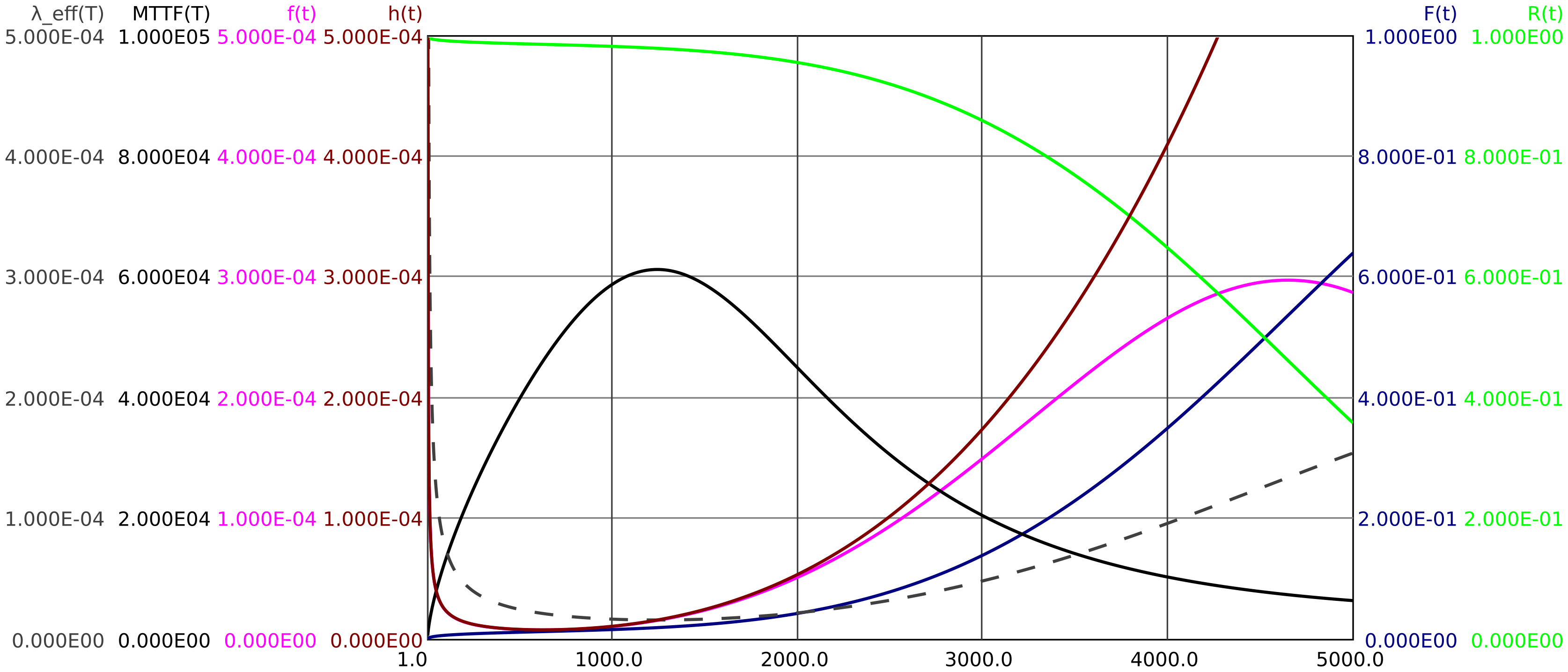
In Figure 7, in addition to failure density \(f(t)\), failure rate \(h(t)\), reliability \(R(t)\) and unreliability \(F(t)\), the effective \(\mathrm {MTTF}(T)\) and (dashed) the effective failure rate \(\lambda _{\mathrm {eff}}(T)\) are also shown as a function of time to preventive replacement \(T\).
It can be seen that for a replacement interval \(T\) of about 1200 hours, the MTTF(T) reaches its maximum of about 61000 h. If the timing belt is changed after about 1200 hours, the effective failure rate is \(\lambda _{\mathrm {eff}}\approx \SI {1.6e-5}{\per \hour }\). If the belt is changed more frequently, the effective (incomplete) MTTF(T) decreases, since early failures still have a relatively strong influence. If the belt is operated for a longer time, the effective MTTF(T) also decreases, as failures due to wear become more noticeable. Preventive replacement should therefore be prescribed after about 1200 hours (or a corresponding distance).
The effective MTTF(T) of 61000 h at a replacement interval of 1200 h practically means, that only about one out of fifty (61000 h/1200 h\(\approx \)50) belts will break in service. 3.
3.3 Dangerous and non-dangerous failure modes, dangerous MTTF
As said already, most components can fail in different ways. In safety related applications, certain failure modes will be safety-critical, others will go to the safe side. For safety considerations, it is therefore often necessary to distinguish between dangerous (d) and safe (s) failure modes. The total failure rate at any time t is the sum of two partial failure rates for dangerous and non-dangerous failures:
\(\seteqnumber{0}{}{29}\)\begin{equation} h(t) = h_d(t) + h_s(t) \end{equation}
The density can be calculated using
\(\seteqnumber{0}{}{30}\)\begin{align} \begin{split} f(t) &= h(t) \cdot R(t) = \big ( h_d(t) + h_s(t) \big ) \cdot R(t) \\ &= h_d(t) \cdot R(t) + h_s(t) \cdot R(t) \\ &= \varphi _d(t) + \varphi _s(t) \end {split} \end{align} into two partial failure densities \(\varphi _d\) and \(\varphi _s\) (\(\varphi _d\) and \(\varphi _s\) are not themselves densities, since their individual integrals are less than 1).
Accordingly, one can decompose the distribution function \(F(t)\) into two subfunctions:
\(\seteqnumber{0}{}{31}\)\begin{equation} F(t) = \Phi _d(t) + \Phi _s(t) = \int \limits _0^t \varphi _d(\tau )\,d\tau + \int \limits _0^t \varphi _s(\tau )\,d\tau \end{equation}
From similar considerations as for the incomplete \(\mathrm {MTTF}(T)\) one obtains for the effective dangerous \(\mathrm {MTTF_d}(T)\):
\(\seteqnumber{0}{}{32}\)\begin{equation} \mathrm {MTTF_d}(T) = \frac {\int \limits _0^T t\cdot f(t)\,dt + T \cdot R(T)}{\Phi _d(T)} \end{equation}
Using the already known formulas for the relationship between reliability and failure rate, we obtain a formula for calculating \(\mathrm {MTTF_d}(T)\) for given or experimentally determined failure rate functions \(h(t)\) and \(h_d(t)\):
\(\seteqnumber{0}{}{33}\)\begin{align} \begin{split} \mathrm {MTTF_d}(T) &= \frac {\int \limits _0^T t\cdot f(t)\,dt + T \cdot R(T)} {\int \limits _0^T \varphi _d(t)\,dt} = \frac {\int \limits _0^T t\cdot h(t) \cdot R(t)\,dt + T \cdot R(T)} {\int \limits _0^T h_d(t) \cdot R(t)\,dt} \\ &= \frac {\int \limits _0^T t\cdot h(t) \cdot \mathrm {e}^{-\int \limits _0^t h(\tau )\,d\tau } \,dt + T \cdot \mathrm {e}^{-\int \limits _0^T h(t)\,dt} } {\int \limits _0^T h_d(t) \cdot \mathrm {e}^{-\int \limits _0^t h(\tau )\,d\tau } \,dt} \end {split} \end{align} A simple formula comparison further yields the relationship:
\(\seteqnumber{0}{}{34}\)\begin{equation} \mathrm {MTTF_d}(T) = \mathrm {MTTF}(T) \frac { F(T) }{ \Phi _d(T) } \end{equation}
Again, the effective mean dangerous failure rate \(\lambda _{\mathrm {d}}\) can be calculated as the reciprocal:
\(\seteqnumber{0}{}{35}\)\begin{equation} \lambda _{\mathrm {d}}(T)=\frac {1}{\mathrm {MTTF_d}(T)} \end{equation}
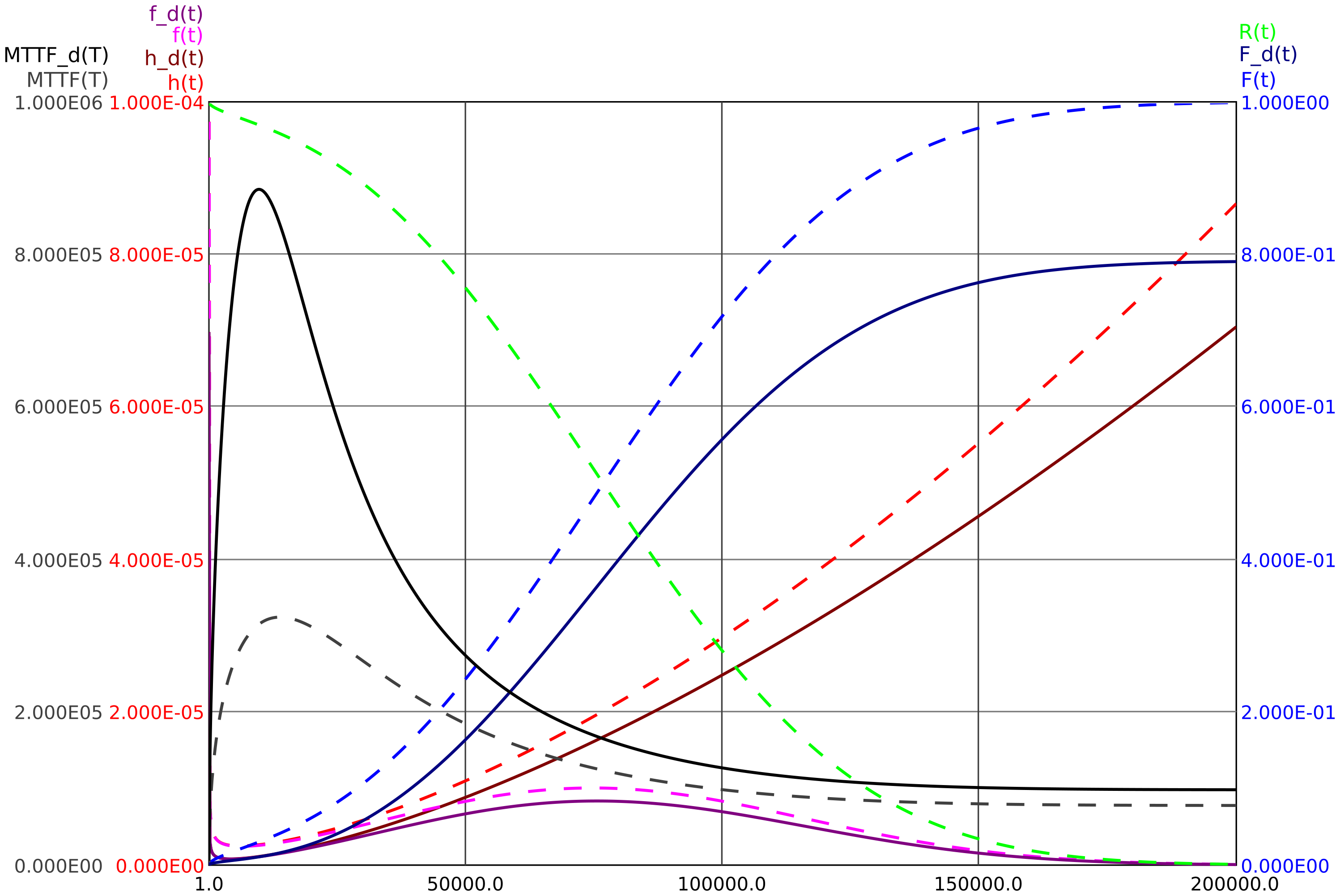
The following figure 8 shows the reliability parameters relevant for a component with three dangerous and three non-dangerous failure types (solid lines for dangerous failures, dashed lines for total failures):