Calculations for Functional Safety
Quantities, Formulas and Methods
6 Failure rate of complex functions
The failure rate is the essential quantity for safety functions, that are required continuously or at least frequently (quasi-continuously). Examples of systems that implement continuously required safety functions, are aircraft engines (shall always provide the required thrust and, most importantly, shall not falsely stall), position control systems (shall always ensure the specified position), drive controls (shall always provide required torques, speeds or positions, or shall not start untimely), railroad signaling systems (shall never indicate a too permissive signal term or give a too permissive drive command) but also airbag controls (shall never falsely trigger the airbag), ABS controls (shall never reduce brake pressure too much), Train door controls (shall never open the door at the wrong time). As soon as the safety function fails there is an immediate dangerous situation. The word "immediate" does not mean, that damage must necessarily occur, but only, that under normal external conditions, damage is not improbable. 14.
Examples of systems that implement quasi-continuously required safety functions, include aircraft landing gears (only need to function during landing, but landing is inevitable), brakes of all vehicles (need to function only when brakes are requested, but the request is almost certain to come – only in exceptional cases coasting to standstill will be possible).
The principle structure of such safety functions is shown in Figure 21.
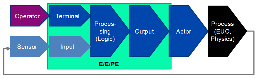
Characteristically, a failure of the safety function directly affects the behavior of the physical process (which is given, for example, by the equations of motion of the vehicle, the aircraft, of the machine or the reaction dynamics of the chemicals and apparatuses) and thus leads to the hazard – regardless of whether the damage occurs immediately or after a foreseeable time.
For continuous safety functions, the concept of process fault tolerance time (PFTT, also called process safety time) is existential: This is the time for which the safety function may be violated, without this resulting in a hazard. In the case of a highly dynamic drive control system or the attitude control system of a fighter jet, this is a maximum of a few milliseconds, in the case of a brake, it may be a few seconds, in the case of the fuel supply of a large power plant, perhaps a few minutes. Any diagnostic measures that may be in place must detect the fault within this time and initiate an adequate response, for example, initiate a safety shutdown or isolate the defective control or actor and activate a redundant control path. A mere error message to the operator is usually not sufficient for continuous or quasi-continuous safety functions, since the operator usually cannot restore the function before the damage occurs.
As with unavailability, the lifetime average of the system failure rate is relevant:
\(\seteqnumber{0}{}{61}\)\begin{equation} \label {eq:overline_h_sys} \overline {h_{\mathrm {sys}}} = \frac {1}{T_{\mathrm {Life}}} \int \limits _0^{T_{\mathrm {Life}}} h_{\mathrm {sys}}(t)\,dt \end{equation}
In [IEC 61508] this mean value \(\overline {h}\) is called Probability of Failure per Hour (PFH for short). 15.
At the top level, \(\overline {h_{\mathrm {sys}}}\) represents the hazard rate, often abbreviated as HR (for hazard rate) (cf. [EN 50126]). If the system under consideration is only a sub-function of a safety function, \(\overline {h_{\mathrm {sys}}}\) is accordingly called Functional Failure Rate (FFR).
\(\overline {h_{\mathrm {sys}}}\) is the relevant measure of safety for all safety functions, the failure of which can lead to damage without further conditions (i. e., safety functions with continuous or at least frequent demand).
Remark: Many controllers perform both continuous safety functions and rarely required ones. In this case, the control system must take into account both the unavailability in the request case \(\overline {Q}\) as well as the frequency of a wrong command to the actuators \(\overline {h}\) must be determined. 16.
14 In contrast to safety functions with rare requests, which are only needed at all in the case of an uncommon external condition (request)
15 Note: Some formulas in the informative Appendix B in [IEC 61508-6] are inconsistent with this, however, the meaning of PFH as a synonymous term to \(\overline {h}\) as defined here is obvious from the rest of the standard and is the only reasonable definition
16 In general, two different fault trees or Markov models are necessary for this, since in particular the diagnosis concerning \(\overline {Q}\) differs from that for \(\overline {h}\), and therefore different basic events (based on a different FMEDA) are needed, and often also different gates
6.1 Calculation with fault trees
The calculation of the failure rate \(\overline {h}\) is much more difficult than the calculation of the unavailability \(\overline {Q}\), both in terms of establishing a correct fault tree and in terms of the actual mathematical calculation. Nevertheless, for most safety functions, fault tree analysis is a suitable method for determining the failure rate, and often the only practicable method of modeling. Unfortunately, however, there is no standardization for this 17 although the essential mathematical principles are already mentioned in [NUREG]. Therefore, it is essential that the analyst familiarizes himself intensively with the properties and peculiarities of the tool used, and, in case of doubt, to convince himself of the correct function of the tool by means of simple tests. The following examples can be the basis of such tests.
17 [EN 61025] does not specify how fault trees can be used to calculate failure rates – neither in terms of modeling nor in terms of calculation.
6.1.1 System without redundancies
In the simplest case, the safety function is realized by a number \(n\) of components, which are all mandatory for the safety function. If one component fails, the safety function fails. The fault tree consists only of OR gates.
-
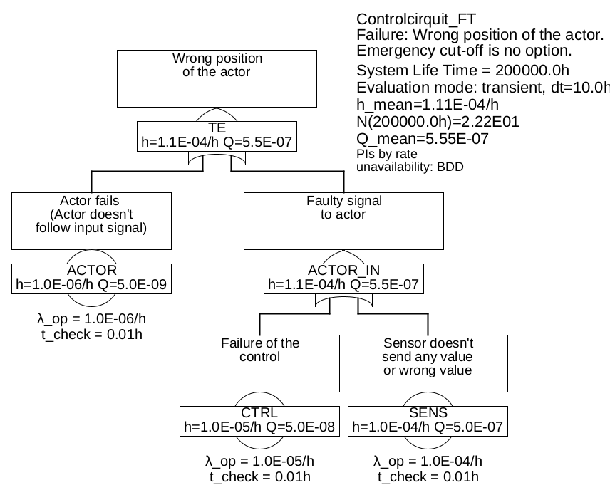
Example 6.1 The fault tree shown in Figure 22 describes such a system, which consists of the components sensors, control and actuators. Here it is assumed that the system must run continuously, there is no possibility of an emergency shutdown in case of detected errors. This is often the case, for example, an aircraft cannot simply be brought to a safe state if the speed sensor system is detected as faulty, because this is absolutely necessary for the flight to continue until landing.
If one of these \(n\) components fails in a dangerous way 18, the safety function is no longer guaranteed. The minimal cuts are obvious: {SENS}, {CTRL}, {ACTOR}.
For the total failure rate, the formula already known from section 3 applies
\(\seteqnumber{0}{}{62}\)\begin{equation} h(t) = \sum _{i=1}^n h_i(t) \end{equation}
Since every fault leads directly to failure, neither system lifetime nor fault detection or repair times play a role, but only the failure rates of the components.
If we assume constant failure rates for all components, the above formula also gives the average failure rate, with the values given in the fault tree thus \(h(t)=\mathrm {const}=\overline {h} =\SI {1.0e-6}{\per \hour }+\SI {1.0e-5}{\per \hour }+\SI {1.0e-4}{\per \hour }=\SI {1.11e-4}{\per \hour }\).
This example was undoubtedly trivial, and hardly anyone would think of to construct a fault tree (or a Markov model) for such a system.
6.1.2 System with redundancies
Fault trees only become really interesting and almost indispensable as a model for systems with redundancies (multi-channel). In the case of redundancies, not every single failure leads to the failure of the safety function, the fault tree will therefore contain at least one AND gate and there will be at least one minimum cut, which contains more than one basic event, i. e. has an order greater than one.
-
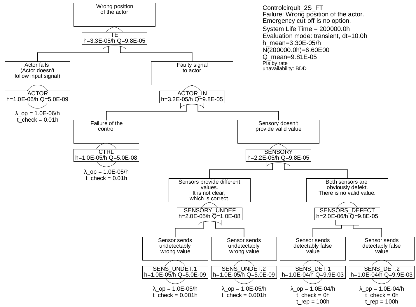
Example 6.2 In example 6.1 the sensor system is obviously a weak point. Therefore, two sensors will now be used in a redundant arrangement, i. e. in such a way that both sensors measure the same physical quantity. As already in example 6.1 let it be assumed, that the system must be running, there is no possibility of an emergency shutdown in case of detected errors.
If a sensor delivers no values at all or obviously wrong values, the measured value of the other sensor can now be used. However, if it is not clear which of the two sensors is defective, the controller still cannot calculate a correct signal for the actor. The same also applies in the case that one sensor is known to be defective, and now the second one fails before the first one has been repaired.
The sensors must therefore now be distinguished with regard to their failure modes: There are defects of the sensors which can be detected by the control system (SENS_DET, such as wire breakage), and those which cannot be detected by the controller (SENS_UNDET). The corresponding fault tree is shown in figure 23.
The minimum cuts are:
-
• {AKTOR}
-
• {CTRL}
-
• {SENS_UNDET.1}
-
• {SENS_UNDET.2}
-
• {SENS_DET.1& SENS_DET.2}
The question now is how to calculate the occurrence rate \(h_{\mathrm {MCS}}(t)\) of the minimal cut {SENS_DET.1 & SENS_DET.2}. The statement of this minimum cut is the following:
-
1. Sensor 1 is known to be defective (i. e. not available, \(Q_{\mathrm {SENS\_DET.1}}\)), and now sensor 2 also fails (with failure rate \(\lambda _{\mathrm {SENS\_DET.2}}\))
OR -
2. Sensor 2 is known to have failed (so not available, \(Q_{\mathrm {SENS\_DET.2}}\)), and now sensor 1 also fails (with failure rate \(\lambda _{\mathrm {SENS\_DET.1}}\)).
Therefore, the minimum cut can be calculated by 19
\(\seteqnumber{0}{}{63}\)\begin{equation*} h_{\mathrm {MCS}}(t) \lessapprox \lambda _{\mathrm {SENS\_DET.1}}\cdot Q_{\mathrm {SENS\_DET.2}}(t) + \lambda _{\mathrm {SENS\_DET.2}}\cdot Q_{\mathrm {SENS\_DET.1}}(t) \end{equation*}
For the events SENS_DET.x the unavailability is needed as well. According to formula (48), this generally depends on the time to detection and the repair time. Since in these events only the failures are considered, which are immediately detectable, the detection time is modeled to zero. The repair time is the time for which the other sensor must hold out, either until a safe condition is reached (e. g. the aircraft has landed) or until a repair has been made while the aircraft is in operation. It is assumed here to be 100 h.
With formula (47) applies
\(\seteqnumber{0}{}{63}\)\begin{equation*} \overline {Q} \approx \lambda \cdot \mathrm {MRT} = \SI {1e-4}{\per \hour } \cdot \SI {100}{\hour }= \num {0.01} \end{equation*}
and thus for the minimum cut
\(\seteqnumber{0}{}{63}\)\begin{equation*} h_{\mathrm {MCS}}(t)=\overline {h_{\mathrm {MCS}}} =\SI {1e-4}{\per \hour }\cdot \num {0.01}+\SI {1e-4}{\per \hour }\cdot \num {0.01}=\SI {2e-6}{\per \hour } \end{equation*}
Since the failure rates of the other minimum cuts are also constant, the total failure rate of the system is therefore
\(\seteqnumber{0}{}{63}\)\begin{equation*} h_{\mathrm {sys}}=\SI {1e-6}{\per \hour }+\SI {1e-5}{\per \hour }+2\cdot \SI {1e-5}{\per \hour }+\SI {2e-6}{\per \hour }=\SI {3.3e-5}{\per \hour } \end{equation*}
-
19 for exactness, see comment on formula (64)
The formula used in the example for the occurrence rate of a minimum cut can be extended to minimum cuts of any order \(m=n_{\mathrm {Lit}}\):
\(\seteqnumber{0}{}{63}\)\begin{equation} \label {eq:h_mcs} \begin{split} h_{\mathrm {MCS}}(t) & \lessapprox h_{1}(t) \cdot Q_{2}(t) \cdot Q_{3}(t) \cdot \ldots \cdot Q_{m}(t) \\ & + h_{2}(t) \cdot Q_{1}(t) \cdot Q_{3}(t) \cdot \ldots \cdot Q_{m}(t) \\ & + \dots \\ & + h_{m}(t) \cdot Q_{1}(t) \cdot Q_{2}(t) \cdot \ldots \cdot Q_{m-1}(t)\\ &=\sum _{j=1}^{m} \left ( h_j(t) \cdot \prod _{k=1,k\neq j}^{m} Q_{k}(t) \right ) \end {split} \end{equation}
Formula (64) is correct only for \(Q_i \rightarrow 0\). The exact formula for two events with arbitrarily large unavailabilities is derived in Example 6.7. However, the error only becomes significant for large unavailabilities, so for correctly designed systems (i. e., when the detection and repair times are much smaller than the MTTF). Moreover, the formula is always conservative, so that even for incorrectly designed systems the failure rate is not estimated too small.
For the system failure rate (or more generally: the occurrence rate of the top event), the following applies
\(\seteqnumber{0}{}{64}\)\begin{equation} \label {eq:h_sys_mcs} \begin{split} h_{\mathrm {sys}}(t) &\lessapprox h_{\mathrm {MCS 1}}(t) + h_{\mathrm {MCS 2}}(t) + \ldots + h_{\mathrm {MCS n}}(t)\\ &= \sum _{i=1}^{n_{\mathrm {MCS}}} \left ( \sum _{j=1}^{n_{\mathrm {Lit,MCS_i}}} \left ( h_j(t) \cdot \prod _{k=1,k\neq j}^{n_{\mathrm {Lit,MCS_i}}} q_{i,k}(t) \right ) \right ) \end {split} \end{equation}
This formula is valid exactly only, if all minimum cuts consist of only one event. Otherwise it can be that the minimum cuts overlap each other, so that the result is somewhat too large. This can be taken into account by disjunction of the minimum cuts as in the calculation of the system unavailability. However, this operation is very time-consuming and reaches the performance limits of modern PCs for large fault trees even when BDDs are used.
6.1.3 Single Channel Fail-Safe
In the last example, it was assumed that the process cannot simply be switched off and brought into a safe state, if an fault is detected. For many processes, this is quite possible, for example, a train can still be brought to a safe stop if the speed measurement fails. It is not even necessary to know exactly which component has failed, but it is also possible to request the safe state in case of inconsistencies of any kind. This will be illustrated in the next example.
Occasionally one speaks of a fail-safe architecture, if the control system is able to to bring the process into a safe state in case of detected failures. However, the term is extremely fuzzy, because there’s no definition which failure modes or what proportion of dangerous failure modes must be detected, in order for a system to be called "fail-safe". 20.
-
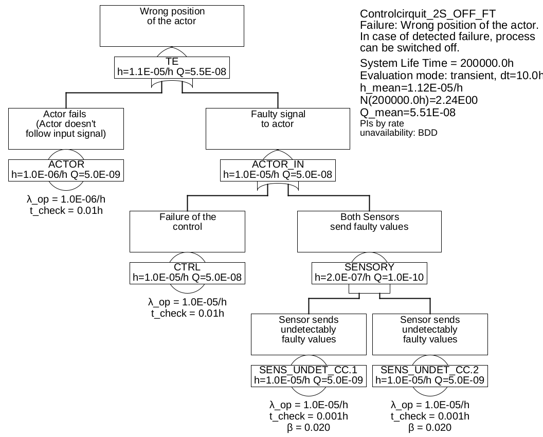
Example 6.3 In this example it is assumed that the control system controls the actor in such a way, that the process goes to a safe state (for example, switching off the power supply or applying the brakes).
In this case, the detectable failures of the sensors SENS_DET are no longer dangerous and can therefore be ignored. And also the situation that a sensor delivers wrong values, but it is not clear which one, is not critical, because in case of a discrepancy, the control system will also control the actuator in such a way that the process reaches a safe state.
The only dangerous case regarding the sensors is the case, that both sensors deliver unrecognizable wrong values at the same time, i. e. the failures SENS_UNDET.1 and SENS_UNDET.2 are present at the same time, and the wrong values are so similar, that they are not recognizable as faulty by the control. So the two failures would not only have to be similar in detail, but also happen so fast one after the other, that this would not be visible to the control system, i. e. typically within the process fault tolerance time (PFTT). One may be tempted to assume that such a case will practically never occur. In fact, this case is unlikely to occur due to independent random events, but experience shows that you should always assume the existence simultaneous failures of redundant components due to external circumstances that have not been taken into account. Flight AF447 or the Fukushima disaster are well-known examples of this. In order to model reality as correctly as possible, one should assume a factor for the proportion of common failures due to external circumstances that are not known or not explicitly taken into account. In [IEC 61508] this is called Common-Cause-Factor and is denoted by \(\beta \). In addition, a guideline is given in [IEC 61508] which can be helpful in estimating this factor. Figure 24 shows the fault tree created in this way. Here \(\beta =2\%\) is assumed between the events SENS_UNDET.1 and SENS_UNDET.2 and therefore they are renamed SENS_UNDET_CC.
The minimum cuts and their partial entry rates are listed in table 1.
Table 1: Minimum cuts for example 6.3Minimum cuts Occurrence rate \(\overline {h}\) CTRL 1.0E-05/h AKTOR 1.0E-06/h SENS_UNDET_CC.COM 2.0E-07/h SENS_UNDET_CC.1 & SENS_UNDET_CC.2 9.604E-14/h In this table, SENS_UNDET_CC.COM denotes the common cause event, that both sensors fail simultaneously in an undetectable manner (due to an external event acting simultaneously). Its occurrence rate is \(\beta \cdot \lambda _{\mathrm {SENS\_UNDET\_CC}} = 0.02 \cdot \SI {1.0e-5}{\per \hour } = \SI {2.0e-7}{\per \hour }\).
The failure rate of the sensor system (gate "SENSORY") thus changes from \(\SI {2.2e-5}{\per \hour }\) to \(\SI {2.0e-7}{\per \hour }\).
In general: In modeling, failures, which go directly to the safe side or in case whose occurrence some measure will be taken, that is always available and most likely to bring the process in a safe state, can be omitted. However, it is essential to check whether these measures are actually available and suitable, to achieve a safe state (of the process!) in all cases. In order to be able to carry out this check, it is imperative that all assumed measures and safe states are mentioned and, especially in the case of generic components, are included in the documentation of the product intended for the customer.
For events below AND gates, proper modeling of unavailability is required. This is based on fault detection and recovery times. In addition, it may be necessary to consider simultaneous failures of redundant components, either by common cause factors \(\beta \) or by an explicit basic event.
For correct modeling of diagnostics and inspection, you need knowledge of the physical or technical process in which the safety function is embedded. If this knowledge is not available (e. g. in case of generic safety systems), all assumptions must be documented as conditions regarding the validity of the fault tree and, if necessary, passed on to customers.
6.1.4 Modeling regular tests and diagnosis
In example 6.3 it was assumed, that the process can easily be brought into a safe state. The safety is largely determined by the failure rate of the control system. It is now obvious to add a diagnostic unit which monitors the activity of the control system. If the diagnostic unit detects a fault, the process (e. g. the machine or the process plant), is ordered to a safe state (standstill, idle) via an additional, simple binary emergency actuator (e. g., a relay or a shut-off valve). The basic architecture of such controls or regulators is shown in Figure 25. It is often referred to as single-channel with diagnostics, in short 1oo1D (for 1-out-of-1).
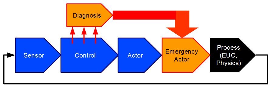
The systematic quality of the diagnostic unit, i. e. the proportion of failures detectable in time by the diagnosis in the total (dangerous) failure modes of the diagnosed component, is called the Diagnostic Coverage (DC). Assuming the diagnostic unit monitors the supply voltages, the processor clock and the regular execution of the critical software tasks (watchdog function), but not the logic of the computing units, the memories, or the input/output units (A/D and D/A converters etc.) of the controller, according to tables in relevant standards, you might get a diagnostic coverage of 70%.
There are now at least three ways to model the diagnosis:
-
1. One decreases the failure rate of the diagnosed component (here CTRL) according to the diagnostic coverage. So the diagnosis does not appear explicitly in the fault tree. The advantage is obviously a simple fault tree. The disadvantage is that the diagnosis is not explicitly mentioned as a safety-relevant component, so it is implicitly assumed that the diagnostics will always work. In fact, however, also the diagnostics and especially the shutdown path is subject to random failures and must therefore be tested regularly in most applications.
-
2. One divides the failures modes of the diagnosed component according to the diagnostic coverage to two basic events, one for the failures not detectable by the diagnosis (CNTRL_UNDET), one for the detectable ones (CTRL_DET).
The failure of the diagnostics itself is also modeled as a basic event (DIAG) with a specific failure rate and test interval. The event for the detectable failures is connected to the diagnostics using an AND gate, cf. Figure 26 left.
-
3. As before, but the basic event of the diagnostic failure is defined as a condition (DIAG_COND), and connected by means of INHIBIT gate to the failure to be diagnosed CTRL_DET), cf. figure 26 on the right.
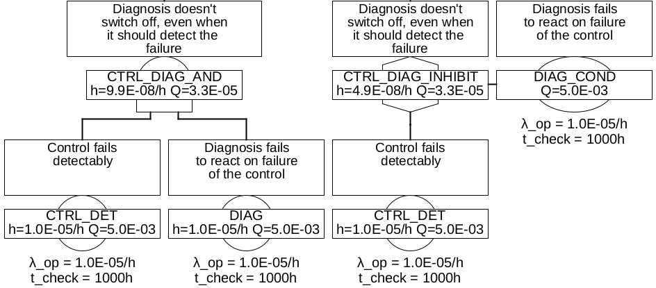
The difference between variants 2 and 3 is the following: With the AND gate, formula (64) applies. Thus, when linking CTRL_DET and DIAG, the result is
\(\seteqnumber{0}{}{65}\)\begin{equation*} h_{\mathrm {AND}} = h_{\mathrm {CTRL\_DET}} \cdot Q_{\mathrm {DIAG}} + h_{\mathrm {DIAG}} \cdot Q_{\mathrm {CTRL\_DET}} \end{equation*}
But this does not reflect the reality, because the failure rate of the diagnosis \(h_{\mathrm {DIAG}}\) has no influence on the occurrence rate of the system failure, but only its unavailability \(Q_{\mathrm {DIAG}}\). Thus, as long as \(Q_{\mathrm {DIAG}}\) is constant, the failure rate of the link should also remain the same. This is achieved by marking an event as a condition, and using INHIBIT to link to the "normal" parts of the fault tree described by occurrence rates \(h\) and unavailabilities \(Q\). Thus, the occurrence rate of the condition is ignored (as if it were zero), and thus the second summand in previous formula becomes zero – exactly what is desired here:
\(\seteqnumber{0}{}{65}\)\begin{equation*} h_{\mathrm {INHIBIT}} = h_{\mathrm {CTRL\_DET}} \cdot Q_{\mathrm {DIAG}} + 0 \cdot Q_{\mathrm {CTRL\_DET}} \end{equation*}
Annotation: The distinction between AND and INHIBIT may be handled with different strictness in different tools, since there is no standardization for this use case either.
Remark: Often, a conditional event is also used to describe the probability, that certain boundary conditions exist. In this case, this probability is entered directly as a constant, see appendix A.3.
Remark: Conditions can be linked together (e. g. by means of AND or OR gates), before they are connected as a total condition to an INHIBIT gate.
-
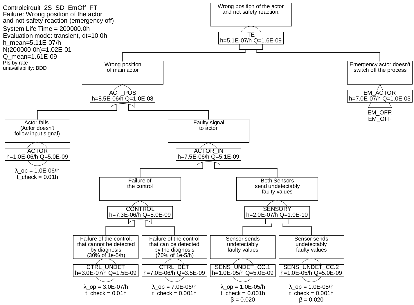
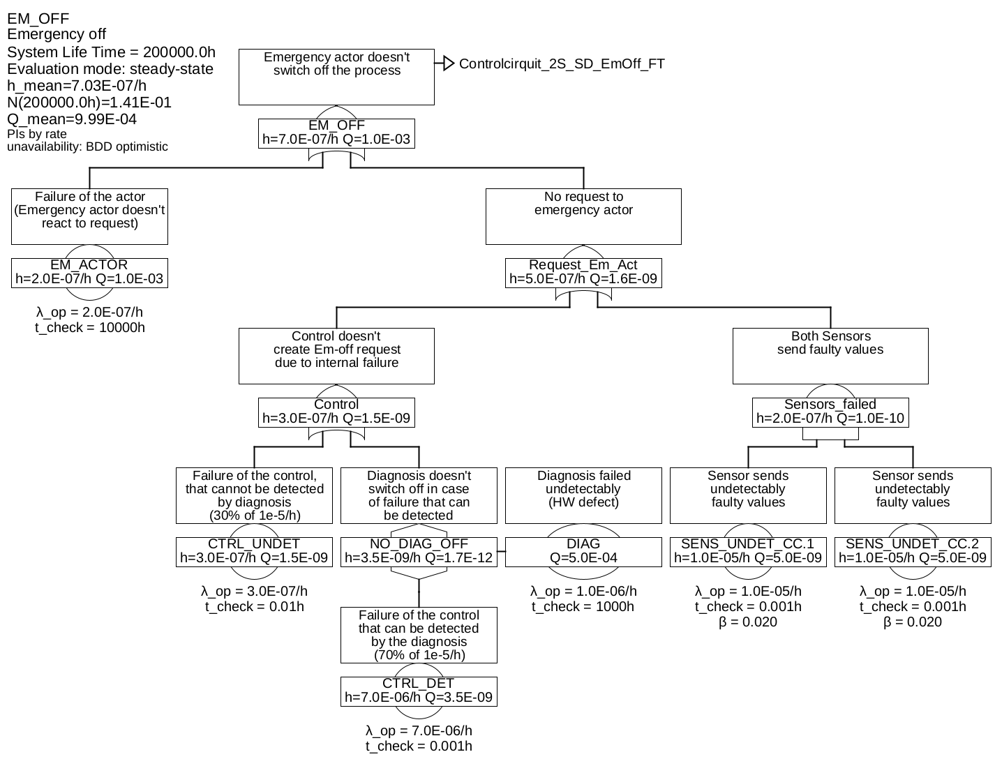
Example 6.4 The figures 27 and 28 represent the fault tree for an architecture, in which the control system is diagnosed and, in the event of a detectable failure, the process is shut down.
The fault tree was split into two partial fault trees to save space. The partial tree for the gate "EM_OFF" was connected to the parent fault tree by means of a transfer gate connected to the parent fault tree. The transfer gate itself has no effect on the calculation, it is only a reference to a branch elsewhere.
It is assumed that the shut-down via the emergency actuator also takes place, if the controller detects that the main actuator is defective. In many applications, it can be easily recognized in time, that the controlled variable increasingly deviates from the set-point, or the control system reads back the manipulated variable (e. g. position of the actor) via an additional input or sensor. The controller can report an actuator fault to the diagnostics simply by putting itself into a failure state that can be clearly recognized by the diagnostics (e. g. no longer resets a watchdog or stops bus communication).
The minimum cuts are listed in table 2.
Table 2: Minimum cuts for example 6.4Minimum cuts Occurrence rate \(\overline {h}\) CTRL_UNDET 3.0E-07/h SENS_UNDET_CC.COM 2.0E-07/h CTRL_DET & EM_ACTOR 6.988E-09/h CTRL_DET & DIAG 3.495E-09/h ACTOR & EM_ACTOR 9.983E-10/h SENS_UNDET_CC.1 & SENS_UNDET_CC.2 9.604E-14/h As soon as there are minimal cuts with more than one event, the unavailability of the events contained therein is relevant, and thus the fault detection and repair times are essential. Therefore, these must be correctly selected and justified, as shown in table 3. The process fault tolerance time was assumed to be 0.01 h.
Table 3: basic events for example 6.4Event Fault detection means
Fault detection time CTRL_UNDET system failure, single fault
irrelevant CTRL_DET diagnosis
0.001 h EM_ACTOR annual test
approx. 10000 h DIAG switch-on self-test after monthly maintenance/cleaning
approx. 1000 h ACTOR control (unexpected process behavior)
0.01 h SENS_UNDET_CC a) difference of sensors
immediately (0.001 h) SENS_UNDET_CC b) Simultaneous failure of both sensors:
considered via common cause \(\beta \), single failureirrelevant The occurrence rate of dangerous failures of the system is now only 5.1E-7/h and is largely determined by the undetected errors of the control system. Further improvements could be achieved by using special safety processors (for example dual-core processors in lock-step mode) and special memory (ECC).
6.1.5 Two-Channel Fail-Safe
The system considered in Example 6.4 is sometimes referred to as a fail-safe single-channel system with diagnostics (1oo1D).
Controllers for high safety requirements are often built up from two individual controllers of the same type, each of which is provided with its own diagnostics. If each of the controls is capable of putting the process to a safe state in the event of a detected fault, this is sometimes referred to as a two-channel fail-safe system, or 1-out-of-2 system with diagnostics, or 1oo2D for short. However, one should use these designations with caution, as they are not harmonized and are used differently and even contradictory in the literature. 21.
21 In [IEC 61508] this architecture is referred to as 1oo2 instead of 1oo2D, since according to this standard a diagnosis must always be present. In part 6 of the standard, 1oo2D is used to refer to a type of fail-operational architecture, which is very unusual and therefore often misunderstood, especially since the accompanying text does not clearly explain this
-
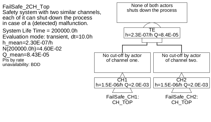
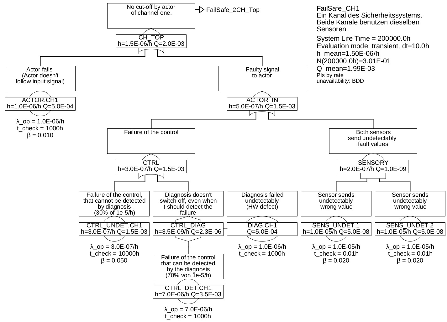
Example 6.5 The fault tree of a two-channel control system, consisting of the sensors already known from the previous examples, which is used jointly by two controllers, each with its own diagnostics and actuator, is shown in figure 29 with the underlying tree shown in Figure 30. Since the channels have the same structure, only the partial fault tree of the first channel is shown.
Each controller can set the process to a safe state via its actuator if faults in the sensory are detected, the diagnostic unit of this channel uses the same actuator for this purpose in case it detects a fault of the controller. At least for undetectable failures of sensors and electronics, as well as failures of actuators, failures due to common causes cannot be excluded. Therefore, not only (as before) the undetectable failures of sensors, but also the undetectable failures of the controllers and the failures of the actuators are provided with common cause factors.
The minimum cuts listed in table 4 can be determined for the system.
Table 4: Minimum cuts for example 6.5Minimum cuts Occurrence rate \(\overline {h}\) SENS_UNDET.COM 2.0E-07/h CTRL_UNDET.COM 1.5E-08/h ACTOR.COM 1.0E-08/h ACTOR.CH1 & CTRL_UNDET.CH2 1.548E-09/h ACTOR.CH2 & CTRL_UNDET.CH1 1.548E-09/h ACTOR.CH1 & ACTOR.CH2 9.699E-10/h CTRL_UNDET.CH1 & CTRL_UNDET.CH2 8.106E-10/h CTRL_UNDET.CH1 & CTRL_DET.CH2 & DIAG.CH2 5.745E-12/h CTRL_DET.CH1 & DIAG.CH1 & CTRL_UNDET.CH2 5.745E-12/h ACTOR.CH1 & CTRL_DET.CH2 & DIAG.CH2 4.542E-12/h ACTOR.CH2 & CTRL_DET.CH1 & DIAG.CH1 4.542E-12/h SENS_UNDET.1 & SENS_UNDET.2 9.604E-13/h CTRL_DET.CH1 & DIAG.CH1 & CTRL_DET.CH2 & DIAG.CH2 2.393E-14/h From table 4 it is clear, that the common cause failures are the major events. This is not unique to this example, but corresponds to practical experience. For this reason, a common cause analysis must always be performed for multichannel systems, and a variety of measures must be taken to keep the rate of common cause failures (mathematically described by the \(\beta \) factor) as low as possible.
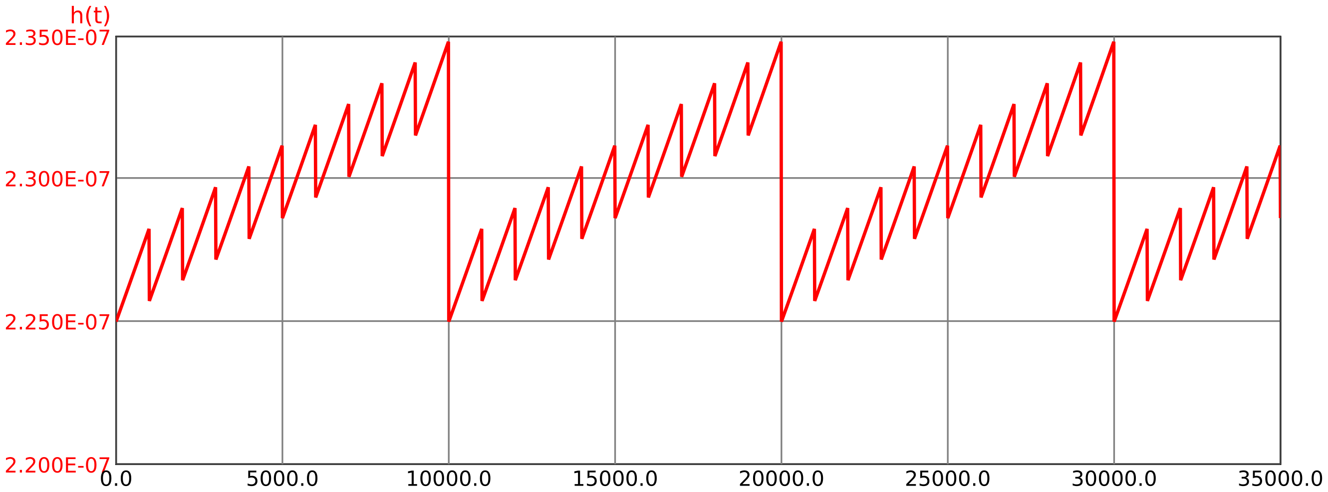
The progression of the failure rate over time is shown in Figure 31.
At first glance, it may seem surprising that the failure rate of the system is not constant, although the failure rates of all components are constant. This is due to the time-varying unavailability of each channel, which is included in the failure rate according to formula (64). Due to the high common cause fractions (see minimum cuts in Table 4), which are directly – without multiplication with an unavailability – included in the system failure rate, the time dependence is, however, only small (note the scale for \(h(t)\) in Figure 31).
6.1.6 Fail operational systems
As mentioned in the introductory example 6.1, there are a large number of processes that cannot simply be brought into a safe state.
If the safety requirements are not very high a two-channel architecture is often sufficient, whereby, in the event of a detected fault, each channel can switch itself off or declare itself defective to a selection circuit. A good self-diagnosis of each channel is essential for this, because only if it is clear which channel is defective, it is possible to switch over to the intact channel. The switchover itself must be performed by a selection circuit.
For higher safety requirements, the diagnostic coverage of the channel-internal diagnostics of the individual channels is often not sufficient, so there is too high a rate of contradictory output from the individual channels, without a channel indicating that it is defective. In this case, the selection circuit would have a 50% chance, of selecting the correct one. The probability of turning off the correct channel, can be improved considerably, by comparing the outputs of three channels. Provided that systematic errors and failures due to common cause are sufficiently rare, usually at least two channels will determine the correct output quantity. The selection circuit is therefore constructed in such a way that it uses the results of the two channels whose results are identical or at least closest to each other. Such an architecture is called a 2-out-of-3 architecture (2oo3, or 2oo3D if each channel has its own diagnostics). 22.
Regardless of the number of channels, the selection circuit must have a minimum failure rate, in order not to limit the overall safety by its own failures. Sometimes the selection is also made by the mechanics, for example, in which each of three channels drives one actuator, which can be mechanically overridden by two others. With appropriate "intelligence" of the selection circuitry, a 2oo3 system can still operate correctly even with two failed channels, if the failures are detected by the channel diagnostics and reported to the selection logic.
22 In contrast to 1oo2, 2oo2, 1oo3, 3oo3, confusion is not possible with 2oo3, because each view gives the same result
-
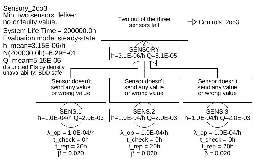
Example 6.6 This example reuses the components of example 6.1. However, now three sensors and three controllers (computers) are used, in such a way that each of the controllers gets the values of all three sensors. Thus, if one sensor fails, all three controllers can continue to operate, in contrast to an architecture where each controller would only have access to one sensor. In addition, each controller can detect sensor faults. The signals for the single actuator calculated by the three controllers are compared by a selection logic and selected according to majority decision (2-of-3).
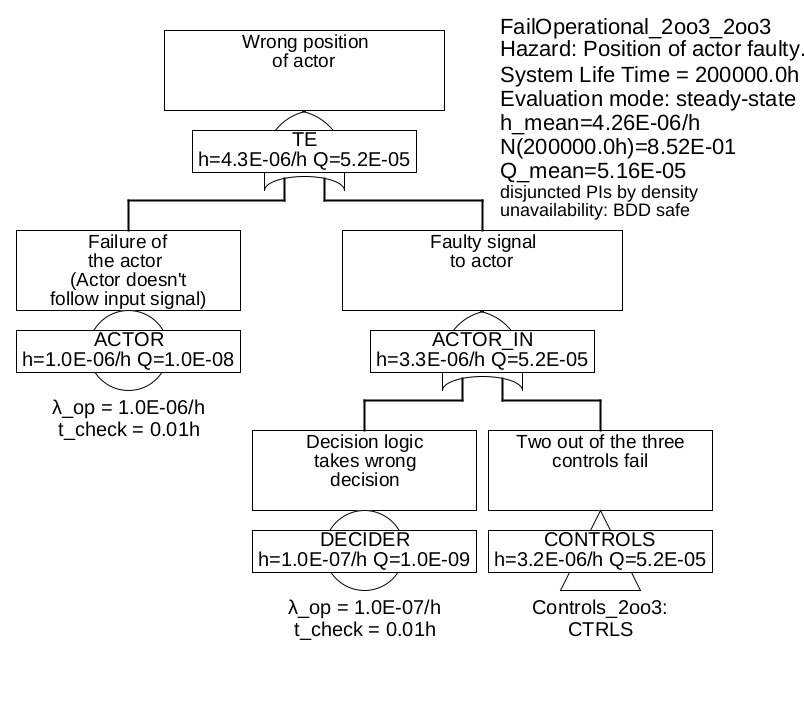
The fault tree is shown in Figure 32, with the sub-trees in 33 and 34.
The "CTRLS" gate in Figure 33 and "SENSORY" in Figure 34 are combination gates, they are explained below.
In addition to the failure rates of all components, the unavailabilities of the controls and the sensors are relevant. Here it was assumed that all failures of the controls as well as all independent failures of the sensors reveal themselves immediately by discrepancies in the selection unit, so the detection time \(t_{\mathrm {test}}\) is zero. The time to repair, i. e., the time that the remaining channels must endure, was assumed to be 20 h (think for example of a long distance airplane, which can only be repaired after landing, or a ship, where the repair of an aggregate is done at sea, but takes a while).
The minimum cuts are listed in table 5.
Table 5: Minimum cuts for example 6.6Minimum cuts Occurrence rate \(\overline {h}\) SENS.COM 2.0E-06/h ACTOR 1.0E-06/h SENS.1 & SENS.2 3.842E-07/h SENS.1 & SENS.3 3.842E-07/h SENS.2 & SENS.3 3.842E-07/h DECIDER 1.0E-07/h CTRL.1 & CTRL.2 4.0E-09/h CTRL.1 & CTRL.3 4.0E-09/h CTRL.2 & CTRL.3 4.0E-09/h The total failure rate has decreased from 1.11E-4/h to 4.26E-6/h compared to example 6.1, and is now mainly determined by sensor failures due to common cause (\(\beta \) was assumed to be 2%).
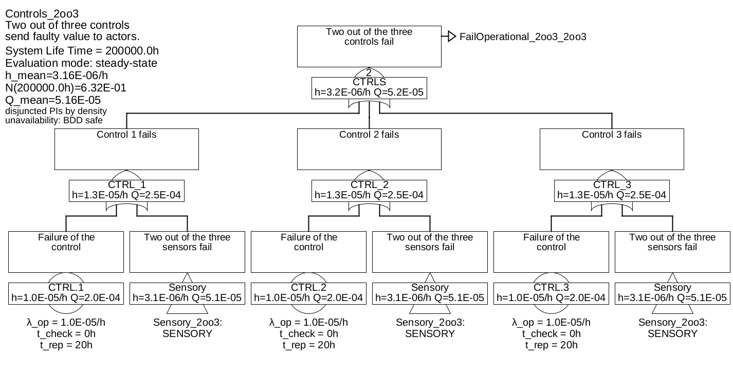
In the previous example, so-called COMBINATION-Gates, also called voting gates, were used for the gates "control" and "sensory". They are just an abbreviation for the corresponding combination of AND and OR gates. The number in the gate (often abbreviated \(m\), so here \(m=2\)) indicates, how many of the \(n\) inputs must fail at least (i. e. must be fulfilled), so that the event described by the gate occurs. Thus \(m=1\) means a pure OR gate, \(m=n\) means a pure AND gate, \(1<m<n\) means a combination of an OR with several AND gates, as shown in Figure 35 as an example for a 2-of-3 gate.
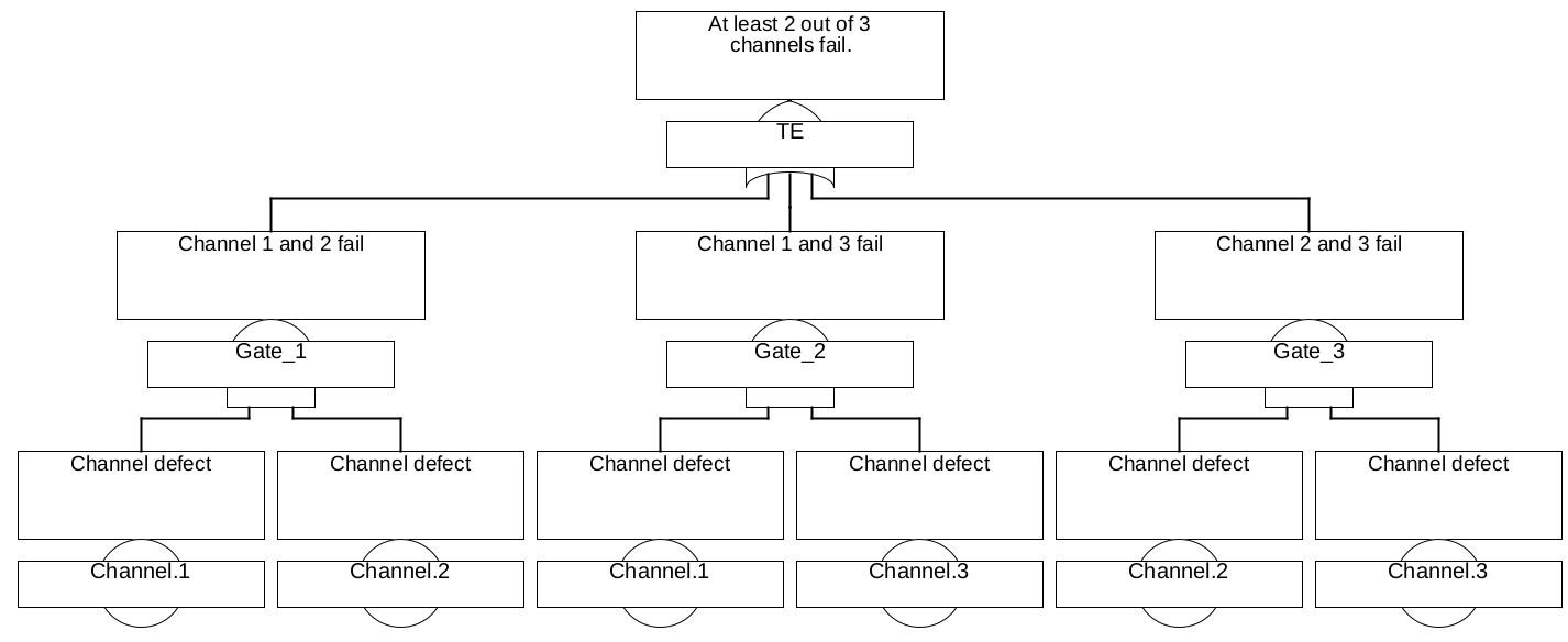
For calculation, the combination gates are converted into the corresponding combination of AND and OR gates. Therefore, there are no special formulas or calculation methods for these gates.
6.1.7 Transient and steady-state calculation
Like the mean system unavailability (see section 5.1.4), the mean system failure rate can also be determined using either a steady-state calculation or a transient calculation.
The only difference is, that the mathematical error described in section 5.1.4 when using mean values only occurs for third order minimal cuts (i. e. minimal cuts with three or more basic events) in calculation of the failure rate, and not already for second-order minimum cuts as in the case of unavailability. This is due to the fact that according to formula (64) for a minimal cut of second order no multiplication of unavailabilities occurs yet. So if it is clear that the system is (apart from a negligible transient phase compared to the operating time) will be in a quasi-stationary state, the system failure rate can usually be calculated in good approximation with mean values.
6.2 Calculation with Markov models
Regarding the modeling there are no differences to chapter 5.2.
As for the calculation of the unavailability, first either the steady state must be calculated, or the linear differential equation system must be integrated over the lifetime.
The occurrence frequency \(w_i(t)\) of a state \(i\) is the sum of the \(m\) transition rates \(h_{i,j}\), which lead to this state, each multiplied by the residence probability in the original state of the respective edge \(p_{\mathrm {Origin}_{i,j}}\):
\(\seteqnumber{0}{}{65}\)\begin{equation} w_i(t) = \sum _{j=1}^m h_{\mathrm {in}_{i,j}}(t) \cdot p_{\mathrm {Origin}_{i,j}}(t) \label {eq:w_state} \end{equation}
The system failure frequency is the sum of the state occurrence frequencies for all \(n\) failure states
\(\seteqnumber{0}{}{66}\)\begin{equation} w_{\mathrm {sys}}(t) = \sum _{i=1}^n w_i(t) = \sum _{i=1}^n \sum _{j=1}^m h_{\mathrm {in}_{i,j}}(t) \cdot p_{\mathrm {Origin}_{i,j}}(t) \label {eq:w_sys} \end{equation}
The failure frequency \(w(t)\) is identical to the searched failure rate \(h(t)\) only, if the residence probability in all failure states is zero, since in practice in the case of a (quasi-)continuously required safety function a system failure is detected practically immediately (namely by the occurrence of an accident), which leads to the immediate termination of operation. Operation is resumed only after the system has been repaired or replaced by another or new one, the time until then must not be taken into account for the calculation of the failure rate (otherwise it would become too optimistic, as can be easily demonstrated with extreme examples).
Thus, if one wishes to use a Markov model to calculate the failure rate \(h_{\mathrm {sys}}(t)\) or \(\overline {h_{\mathrm {sys}}}\), one either has to calculate a transition from all failure states with a very high rate \(\mu \) back to a non-failure state (usually back to the initial state), or one has to divide the failure frequency \(w(t)\) by the probability , of not being in a failure state:
\(\seteqnumber{0}{}{67}\)\begin{equation} \label {eq:h_sys_MM} h_{\mathrm {sys}}(t) = \frac {w_{\mathrm {sys}}(t)}{1-\sum \limits _{i=1}^n p_i(t)} \end{equation}
If the probabilities of the failure states are zero, we get \(h(t) = w(t)\). Formula (68) can and should always be used to be on the safe side, even if – as mentioned before – transitions with large recovery rate \(\mu \) have already been inserted in the model.
-
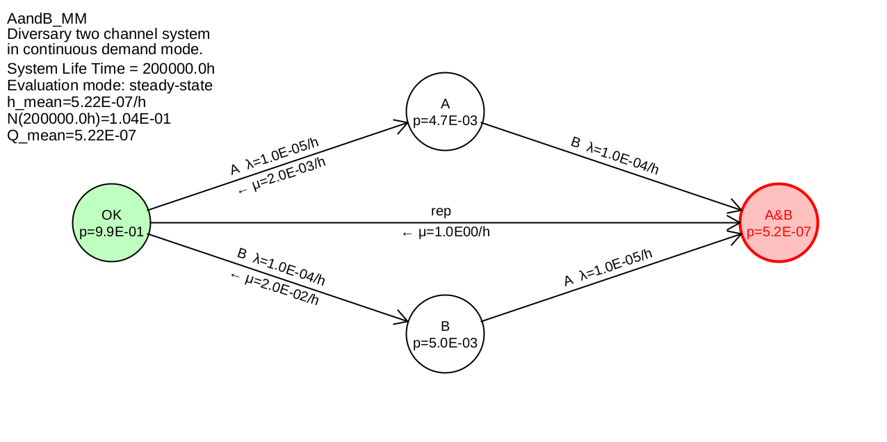
Example 6.7 The above formulas will now be applied to a simple Markov model. For this purpose, a simple diversitary two-channel system is assumed, consisting of the differently constructed (diversitary) channels A and B. Channels A and B therefore have different failure rates \(\lambda _{\mathrm {A}}\) and \(\lambda _{\mathrm {B}}\). Both channels A and B are tested regularly, but at different intervals \(T_{\mathrm {A}}\) and \(T_{\mathrm {B}}\). This results in different \(\mu _A=2/T_{\mathrm {A}}\) and \(\mu _B=2/T_{\mathrm {B}}\).
If both channels fail, the continuously required safety function fails, thus terminates its operation due to an accident. Repairing or replacing the system after an accident leads back to the original OK state. The probability of staying in the A&B state during operation is zero, which is due to a very large \(\mu _{\mathrm {rep}}\) compared to the failure rates.
The associated Markov model is shown in Figure 36.
The transition matrix is:
\(\seteqnumber{0}{}{68}\)\begin{equation*} \label {T} T = \begin{pmatrix} -\lambda _A-\lambda _B & \mu _A & \mu _B & \mu _{\mathrm {rep}}\\ \lambda _A & -\mu _A-\lambda _B & 0 & 0\\ \lambda _B & 0 & -\mu _B-\lambda _A & 0\\ 0 & \lambda _B & \lambda _A & -\mu _{\mathrm {rep}} \end {pmatrix} \end{equation*}
For the stationary calculation one of the lines is set to 1 (here the last one was taken):
\(\seteqnumber{0}{}{68}\)\begin{equation*} \begin{pmatrix} -\lambda _B-\lambda _A & \mu _A & \mu _B & \mu _{\mathrm {rep}} \\ \lambda _A & -\mu _A-\lambda _B & 0 & 0 \\ \lambda _B & 0 & -\mu _B-\lambda _A & 0 \\ 1 & 1 & 1 & 1 \end {pmatrix} \cdot \vec {p}(t) = \begin{pmatrix} 0 \\ 0 \\ 0 \\ 1 \end {pmatrix} \end{equation*}
According to formulas (67) and (68), the system failure occurrence rate results in
\(\seteqnumber{0}{}{68}\)\begin{equation*} h_{\mathrm {sys}} = \frac {p_{\mathrm {A}}\cdot \lambda _{\mathrm {B}}+p_{\mathrm {B}}\cdot \lambda _{\mathrm {A}}}{1-p_{\mathrm {A\&B}}} \end{equation*}
The state probabilities required in this formula \(p_{\mathrm {A}}\), \(p_{\mathrm {B}}\) and \(p_{\mathrm {A\&B}}\) are obtained by solving the system of equations. Thus \(h_{\mathrm {sys}}\) is given by
\(\seteqnumber{0}{}{68}\)\begin{align*} h_{\mathrm {sys}} &= \dfrac {\lambda _{\mathrm {A}}\lambda _{\mathrm {B}}^{2} + \lambda _{\mathrm {A}}^{2}\lambda _{\mathrm {B}} +\lambda _{\mathrm {A}}\lambda _{\mathrm {B}}\mu _{\mathrm {A}} +\lambda _{\mathrm {A}}\lambda _{\mathrm {B}}\mu _{\mathrm {B}} } {\lambda _{\mathrm {A}}^{2}+\lambda _{\mathrm {B}}^{2}+\lambda _{\mathrm {A}}\lambda _{\mathrm {B}} +\left ( \lambda _{\mathrm {a}}+\lambda _{\mathrm {B}} \right ) \mu _{\mathrm {A}} +\left ( \lambda _{\mathrm {A}}+\lambda _{\mathrm {B}} \right ) \mu _{\mathrm {B}} +\mu _{\mathrm {A}} \mu _{\mathrm {B}} } \\ &= \dfrac { \lambda _{\mathrm {A}}\lambda _{\mathrm {B}} \left ( \lambda _{\mathrm {A}} + \lambda _{\mathrm {B}} + \mu _{\mathrm {A}} + \mu _{\mathrm {B}} \right ) } { \lambda _{\mathrm {A}} \left ( \lambda _{\mathrm {A}} + \mu _{\mathrm {A}} + \mu _{\mathrm {B}} \right ) + \lambda _{\mathrm {B}} \left ( \lambda _{\mathrm {B}} + \mu _{\mathrm {A}} + \mu _{\mathrm {B}} \right ) + \lambda _{\mathrm {A}}\lambda _{\mathrm {B}} + \mu _{\mathrm {A}} \mu _{\mathrm {B}} } \end{align*} It should be noted, that the rate \(\mu _{\mathrm {rep}}\) does not appear in the result, since it is truncated by formula (68). This corresponds exactly to the expectation, that the numerical value of this rate must be irrelevant. This formula is now valid for any test interval, in contrast to formula (64), which is only valid for sufficiently small test intervals (otherwise formula (64) becomes somewhat too large).
For suitable test intervals \(T_{\mathrm {test,A}} \ll 1/\lambda _{\mathrm {A}}\) and \(T_{\mathrm {Test,B}} \ll 1/\lambda _{\mathrm {B}}\) , \(\lambda _{\mathrm {A}}\) is negligible vs. \(\mu _{\mathrm {A}}\) and \(\lambda _{\mathrm {B}}\) is negligible vs. \(\mu _{\mathrm {B}}\), and even more so is \(\lambda _{\mathrm {A}}\lambda _{\mathrm {B}}\) negligible vs. \(\mu _{\mathrm {A}} \mu _{\mathrm {B}}\). Thus, we get the conservative approximation:
\(\seteqnumber{0}{}{68}\)\begin{align*} h_{\mathrm {sys}} &\lessapprox \dfrac { \lambda _{\mathrm {A}}\lambda _{\mathrm {B}} \left ( \mu _{\mathrm {A}} + \mu _{\mathrm {B}} \right ) } { \lambda _{\mathrm {A}} \left ( \mu _{\mathrm {A}} + \mu _{\mathrm {B}} \right ) + \lambda _{\mathrm {B}} \left ( \mu _{\mathrm {A}} + \mu _{\mathrm {B}} \right ) + \mu _{\mathrm {A}} \mu _{\mathrm {B}} } \\ &= \dfrac { \lambda _{\mathrm {A}}\lambda _{\mathrm {B}} \left ( \dfrac {1}{\mu _{\mathrm {A}}} + \dfrac {1}{\mu _{\mathrm {B}}} \right ) } { \lambda _{\mathrm {A}} \left ( \dfrac {1}{\mu _{\mathrm {A}}} + \dfrac {1}{\mu _{\mathrm {B}}} \right ) + \lambda _{\mathrm {B}} \left ( \dfrac {1}{\mu _{\mathrm {A}}} + \dfrac {1}{\mu _{\mathrm {B}}} \right ) + 1 } \end{align*}
Under the same condition (suitable test intervals) is also valid \(\lambda _{\mathrm {A}}/\mu _{\mathrm {A}} \ll 1\) and \(\lambda _{\mathrm {B}}/\mu _{\mathrm {B}} \ll 1\) and consequently the approximation:
\(\seteqnumber{0}{}{68}\)\begin{align*} h_{\mathrm {sys}} &\lessapprox \dfrac { \lambda _{\mathrm {A}}\lambda _{\mathrm {B}} \left ( \dfrac {1}{\mu _{\mathrm {A}}} + \dfrac {1}{\mu _{\mathrm {B}}} \right ) } { \dfrac {\lambda _{\mathrm {A}}}{\mu _{\mathrm {B}}} + \dfrac {\lambda _{\mathrm {B}}}{\mu _{\mathrm {A}}} + 1 } \end{align*}
Replacing now the repair rates by the test intervals by \(\mu _{\mathrm {i}} \approx 2/T_{\mathrm {test,i}}\), one obtains
\(\seteqnumber{0}{}{68}\)\begin{equation*} h_{\mathrm {sys}} \approx \dfrac { \lambda _{\mathrm {A}}\lambda _{\mathrm {B}} \left ( T_{\mathrm {Test,A}}+T_{\mathrm {Test,B}} \right ) } { \lambda _{\mathrm {A}} T_{\mathrm {Test,B}} + \lambda _{\mathrm {B}} T_{\mathrm {Test,A}} + 2 } \end{equation*}
Under the additional condition, that the test intervals would also be sufficiently short for the failure rate of the other channel, i. e. \(\lambda _{\mathrm {A}} T_{\mathrm {test,B}} \ll 1\) and \(\lambda _{\mathrm {B}} T_{\mathrm {test,A}} \ll 1\) the products in the denominator can be neglected:
\(\seteqnumber{0}{}{68}\)\begin{equation*} h_{\mathrm {sys}} \approx \lambda _{\mathrm {A}} \lambda _{\mathrm {B}} \dfrac {T_{\mathrm {Test,A}} + T_{\mathrm {Test,B}}}{2} \end{equation*}
This is the formula (64) already known for the calculation of the failure rate of a minimal cut, applied to the single minimal cut of this Markov model {A&B}:
\(\seteqnumber{0}{}{68}\)\begin{equation*} h_{\mathrm {sys}} = h_{\mathrm {MCS}} \lessapprox \lambda _{\mathrm {A}} Q_{\mathrm {B}} + \lambda _{\mathrm {B}} Q_{\mathrm {A}} \lessapprox \lambda _{\mathrm {A}} \lambda _{\mathrm {B}} \dfrac {T_{\mathrm {Test,B}}}{2} + \lambda _{\mathrm {B}} \lambda _{\mathrm {A}} \dfrac {T_{\mathrm {Test,A}}}{2} = \lambda _{\mathrm {A}} \lambda _{\mathrm {B}} \dfrac {T_{\mathrm {Test,A}} + T_{\mathrm {Test,B}}}{2} \end{equation*}
6.3 Expected value of failures
For repairable or replaceable systems, in addition to the failure rate, the expected value of failures \(N(t)\) is also of interest:
\(\seteqnumber{0}{}{68}\)\begin{equation} N_{\mathrm {sys}}(T) = \int \limits _0^T h_{\mathrm {sys}}(t) dt \end{equation}
It indicates how many failures can be expected in the time interval \(t=0\dots T\).
The average failure rate \(\overline {h}\) can also be calculated from \(N(T)\):
\(\seteqnumber{0}{}{69}\)\begin{equation} \label {eq:h_mean_N} \overline {h_{\mathrm {sys}}} = \mathrm {PFH} = \frac {N_{\mathrm {sys}}(T)}{T} \end{equation}