Calculations for Functional Safety
Quantities, Formulas and Methods
4 Recovery and availability
For components and systems, which are repaired or replaced in the event of a failure, further considerations and quantities are required.
4.1 Repairability
If it must be assumed, that during the specified period of use of the overall system, multiple failures of the function may occur, a system (or a function) is repairable. It does not matter whether the system is repaired in the literal sense, or single components or even the whole system is replaced by an equal or different one. Repairability is therefore not a matter of definition (like the definition of a smallest replaceable unit or of total loss), but results inevitably from the reliabilities of the components and the planned service lifetime. The much simpler modeling of a function as non-repairable may only be chosen if the unreliability of all components over the intended, specified service lifetime is small (approximately less than 0.1). This is practically never fulfilled in the case of long-lasting systems such as aircraft, locomotives, machinery or industrial plants, in the case of short-lived systems (such as passenger cars) only for some functions.
4.2 Diagnosis, test, recovery
According to [IEC 61508] and other standards, diagnostics are the measures, that detect a fault within the process fault tolerance time (PFTT, also called process safety time). This is the time that a physical process (e. g., a motor or valve in a machine) is allowed to be incorrectly controlled without resulting in an uncontrollable or dangerous state of the overall system.
Tests are the measures which reveal errors only after a more or less precisely defined fault detection time, for example, in the course of a restart (power-on-self test), a test routine to be performed regularly (test run) or during a maintenance measure (workshop inspection). The average time in which an existing fault is detected, is usually abbreviated to MTTD (Mean Time To Detect). If a test is performed at regular intervals \(T_{\mathrm {test}}\), then the \(\mathrm {MTTD}=T_{\mathrm {test}}/2\).
In case of a detected defect, either the defective component is repaired or replaced, or a whole module is replaced or even the whole system (machine, vehicle,...) is taken out of operation and replaced by a new one. In any case, the function is restored, because this is usually still needed. With which measure the function is concretely restored, is irrelevant for the further considerations.
4.3 Availability and unavailability
Availability \(A(t)\) is the probability, that a component/system/function works at time \(t\).
Unavailability \(Q(t)\) is the probability, that a component/system/function will not work at time \(t\). Consequently, it is the complementary probability to availability:
\(\seteqnumber{0}{}{36}\)\begin{equation} A(t) = 1 - Q(t) \quad \textrm {or} \quad Q(t) = 1 - A(t) \end{equation}
Availability is the decisive variable for systems/functions, which are only required occasionally, in particular functions that are only required in exceptional or emergency cases (e. g. alarms or fire extinguishing devices). It is also an essential quantity for systems/functions which have redundancies, so-called multi-channel systems, more on this later.
For a component or system, which is never tested and therefore never repaired or replaced:
\(\seteqnumber{0}{}{37}\)\begin{equation} Q(t) = F(0,t) \end{equation}
Availability can be significantly increased by continuous diagnostics or regular tests and, if necessary, restoration. This is the reason why most emergency systems are tested regularly.
When a component is tested and repaired or replaced in case of a defect, \(Q(t) = F(t)\) is valid only until the first test. In the case of regular tests at intervals of \(T_{\mathrm {test}}\) the following equation is theoretically valid until the first restoration:
\(\seteqnumber{0}{}{38}\)\begin{equation*} Q(t) = \frac { F(t - t \bmod T_{\mathrm {test}},t) } { R(0, t - t \bmod T_{\mathrm {test}}) } = \frac { F(t) - F(t - t \bmod T_{\mathrm {test}}) }{ R(t - t \bmod T_{\mathrm {test}}) } \end{equation*}
However, since it is not known when the first defect will occur and thus the first repair or replacement will be necessary, this formula is practically meaningless. For the same reason, a variable failure rate is also practically meaningless, because one can never say how long a component has been in use at time \(t\), since one does not know when it was installed – it could already be a replacement. Consequently, a mean failure rate \(\overline {h}=\lambda =1/\mathrm {MTTF}\) must always be determined and used according to section 3.
For components and systems, which are regularly (and completely) tested, the unavailability is a periodic sequence of initial pieces of the exponential distribution, therefore:
\(\seteqnumber{0}{}{38}\)\begin{equation} Q(t) = F(0, t \bmod T_{\mathrm {test}}) = 1-\mathrm {e}^{-\lambda (t \bmod T_{\mathrm {test}} )} \label {eq:q_t_exakt} \end{equation}
If the time \(t\) is small with respect to \(\mathrm {MTTF}=1/\lambda \), then slightly conservatively
\(\seteqnumber{0}{}{39}\)\begin{equation} Q(t) \lessapprox \lambda \cdot (t \bmod T_{\mathrm {test}} ) \label {eq:q_t_approx} \end{equation}
For an average failure rate \(h(t)=\lambda =\SI {1e-5}{\per \hour }\) and a test interval \(T_{\mathrm {test}}=\SI {1000}{\hour }\), unavailability \(Q(t)\) and unreliability \(F(t)\) are shown in Figure 9.
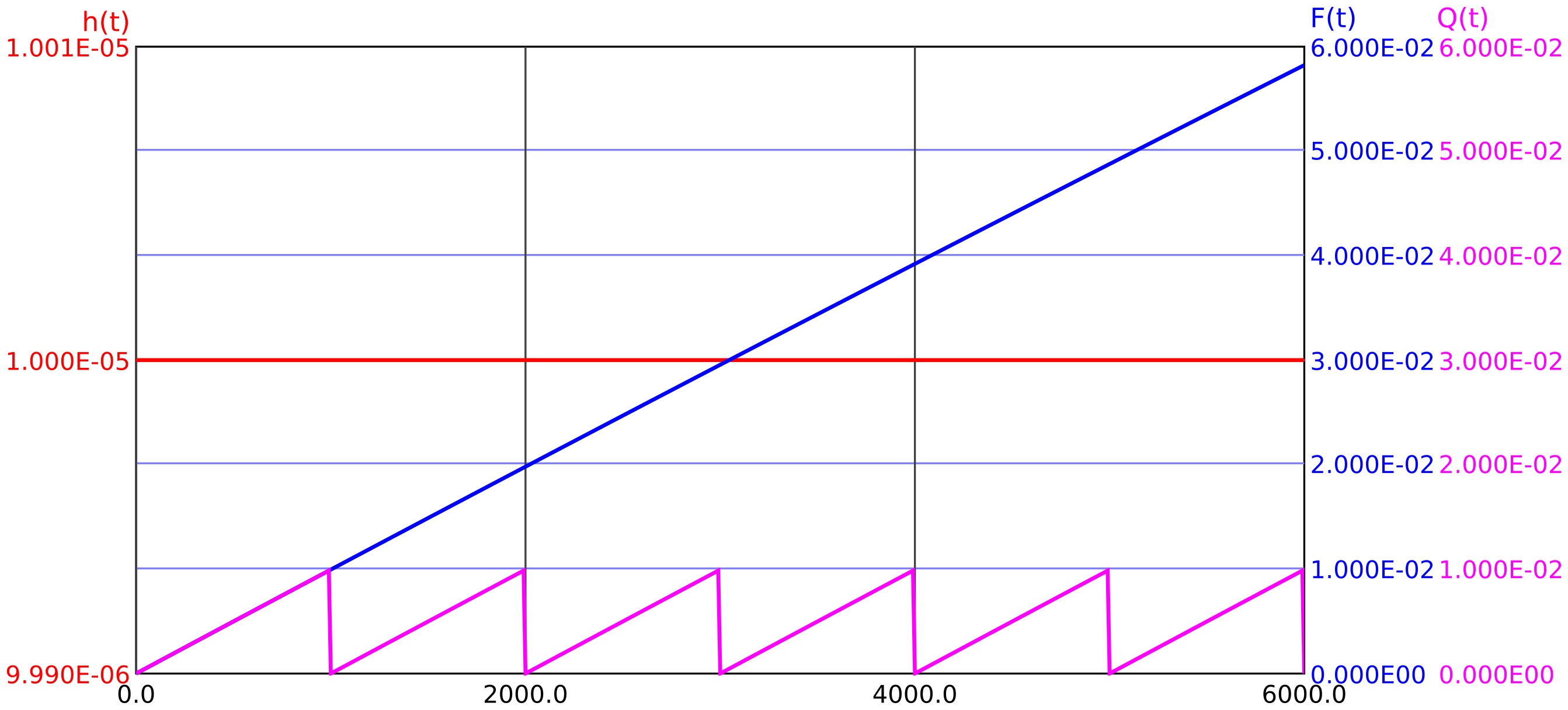
The unavailability decreases to zero with each test, then increases again. It is assumed that the regular test is complete, i. e. reveals all relevant faults of the component. If this is not the case this remaining part must be considered as a further unavailability with a correspondingly smaller failure rate, but longer test time (usually the system lifetime) must be added. Roughly speaking, one can simply add this second unavailability, in special software tools (FTA or Markov tools) an exact treatment is also possible.
-
Example 4.1 A smoke detector has an average failure rate of \(\overline {h(t)}=\lambda =1/\SI {100000}{\hour }=\SI {1e-5}{\per \hour }\). It would be tested annually (every \(T=\SI {8760}{\hour }\)) and replaced if necessary. What is the probability that it will not work in the event of a fire?
The mean unavailability over the test interval \(T_{\mathrm {test}}\) must be determined:
\(\seteqnumber{0}{}{40}\)\begin{equation*} \overline {Q(0..T)} = \frac {1}{T} \int \limits _0^T{1 - \mathrm {e}^{-\lambda \cdot t}} dt = \frac {1}{T} \left ( t + \frac {1}{\lambda } \mathrm {e}^{-\lambda \cdot t} \right ) \Bigg |_0^T = 1 + \frac {\mathrm {e}^{-\lambda \cdot T} - 1}{\lambda \cdot T} = 0.0426 \end{equation*}
When the unavailability is small (say \(Q<\num {0.1}\)), the conservative approximation holds very well:
\(\seteqnumber{0}{}{40}\)\begin{equation} \overline {Q(0..T_{\mathrm {test}})} \lessapprox \num {0.5}\cdot \lambda \cdot T_{\mathrm {test}} \label {eq:q_mean_approx} \end{equation}
In the previous example this would result in \(\overline {Q(0..T_{\mathrm {test}})} \approx \num {0.0438}\) instead of 0.0426.
The unavailability is a probability, it can only take values from 0 to 1, but unlike unreliability, it is monotonically increasing only in the special case of a non-testable/non-repairable) system. After each test, however, unlike unreliability \(F(t)\), the unavailability \(Q(t)\) drops back to zero (or at least to a value close to zero in the case of a noncomplete test).
4.4 Time to repair, MRT
If only a partial function is affected by the defect, the continued operation of the surrounding larger system might be possible (if necessary with restrictions). In that case, the time required for repair and/or replacement (MRT, Mean Repair Time) must also be taken into account in the unavailability. Together with the time to detect the fault (MTTD), this results in the Mean Time To Restore (MTTR):
\(\seteqnumber{0}{}{41}\)\begin{equation} \mathrm {MTTR} = \mathrm {MTTD} + \mathrm {MRT} \end{equation}
For the exact calculation of the mean unavailability, we can start from its definition:
\(\seteqnumber{0}{}{42}\)\begin{align} \label {eq:mean_q_test_rep} \begin{split} \overline {Q} &= \frac {T_{\mathrm {def}}}{T_{\mathrm {overall}}} = \frac { T_{\mathrm {ud}} + p_{\mathrm {def}} \cdot \mathrm {MRT} } {(1-p_{\mathrm {def}}) \cdot T_{\mathrm {test}} + p_{\mathrm {def}} \cdot (T_{\mathrm {test}}+\mathrm {MRT} )} \\ &= \frac { T_{\mathrm {ud}} + p_{\mathrm {def}} \cdot \mathrm {MRT} } { T_{\mathrm {test}} + p_{\mathrm {def}} \cdot \mathrm {MRT} } \end {split} \end{align}
where \(p_{\mathrm {def}}\) denotes the probability, to find the function defective at the regular test time \(T_{\mathrm {test}}\).
\[ p_{\mathrm {def}} = F(T_{\mathrm {test}}) = 1-e^{-\lambda \cdot T_{\mathrm {test}}} \]
and \(T_{\mathrm {ud}}\) the mean time in each test interval, during which the function is undetectably unavailable due to the defect (i. e. the MTTD divided over all test intervals until failure)
\[ \begin {split} T_{\mathrm {ud}} &= \int \limits _0^{T_{\mathrm {test}}} f(t) \cdot (T_{\mathrm {test}} - t)\;dt = \int \limits _0^{T_{\mathrm {test}}} \lambda \cdot e^{-\lambda \cdot T_{\mathrm {test}} } \cdot (T_{\mathrm {test}} - t) \;dt\\ &= \frac {e^{-\lambda \cdot T_{\mathrm {test}}} -1} {\lambda } +T_{\mathrm {test}} \end {split} \]
By substituting in formula (43) we get for the mean unavailability
\(\seteqnumber{0}{}{43}\)\begin{align} \label {eq:q_mean_exact_mttr} \begin{split} \overline {Q} &= \frac { \dfrac {e^{-\lambda \cdot T_{\mathrm {test}}}-1}{\lambda } + T_{\mathrm {test}} + \mathrm {MRT} \cdot ( 1-e^{-\lambda \cdot T_{\mathrm {test}}} ) } { T_{\mathrm {test}} + \mathrm {MRT} \cdot ( 1-e^{-\lambda \cdot T_{\mathrm {test}}} ) } \\ &= \frac { e^{-\lambda \cdot T_{\mathrm {test}}} - 1 } { \lambda \cdot T_{\mathrm {test}} + \lambda \cdot \mathrm {MRT} \cdot ( 1-e^{-\lambda \cdot T_{\mathrm {test}}} ) } + 1 \end {split} \end{align}
For negligible detection time \(T_{\mathrm {test}} \rightarrow 0\) (continuous diagnostics, small test intervals or fault revelation by immediately detectable malfunction) the mean (safety relevant) unavailability approaches
\(\seteqnumber{0}{}{44}\)\begin{equation} \label {eq:q_mean_MRT} \overline {Q} = \frac { \lambda \cdot \mathrm {MRT} } { \lambda \cdot \mathrm {MRT} + 1 } \end{equation}
as obtained by applying de l’Hospital’s rule once to formula (44).
For negligible repair time \(\mathrm {MRT} \rightarrow 0\) (e. g., out of service during repair), formula (44) simplifies directly to
\(\seteqnumber{0}{}{45}\)\begin{equation} \label {eq:q_mean_test} \overline {Q} = \frac {e^{-\lambda \cdot T_{\mathrm {test}}}-1} {\lambda \cdot T_{\mathrm {test}} }+1 \end{equation}
If both test interval \(T_{\mathrm {test}}\) and repair time \(\mathrm {MRT}\) are small vs \(MTTF\), holds with sufficient accuracy
\(\seteqnumber{0}{}{46}\)\begin{equation} \label {eq:q_mean_approx_mttr} \overline Q \lessapprox \lambda \cdot \left ( \num {0.5}\cdot T_{\mathrm {test}} + \mathrm {MRT} \right ) \end{equation}
It is more difficult to derive an (exact) formula for the unavailability at a certain point in time, if the repair time is not negligible. A very good approximation is given by
\(\seteqnumber{0}{}{47}\)\begin{equation} \label {eq:q_t_mttr} Q(t) = 1-\frac { e^{-\;\dfrac {\lambda \cdot (t \bmod T_{\mathrm {test}}) }{ \lambda \cdot \mathrm {MRT} + 1 }} }{ \lambda \cdot \mathrm {MRT} + 1 } \end{equation}
(without derivation). For repair time \(\mathrm {MRT} \rightarrow 0\), formula (48) goes directly to formula (39):
\[ Q(t) = 1-\mathrm {e}^{-\lambda (t \bmod T_{\mathrm {test}} )} \]
For negligible detection time \(T_{\mathrm {test}} \rightarrow 0\) immediately results in
\[ Q(t) = 1-\frac { e^{-\;\dfrac {0}{ \lambda \cdot \mathrm {MRT} + 1 }} }{ \lambda \cdot \mathrm {MRT} + 1 } = 1-\frac {1}{ \lambda \cdot \mathrm {MRT} + 1 } = \frac { \lambda \cdot \mathrm {MRT} } { \lambda \cdot \mathrm {MRT} + 1 } = \overline {Q} \]
thus formula (45).
4.5 Continuous diagnosis
In the case of continuous complete diagnosis (i. e. every error is detected immediately) the unavailability has nothing to do with the (un)reliability, so \(Q(t) \neq F(t)\) is always valid. Unavailability then depends only on the (mean) failure rate \(\overline {h}=\lambda \) and the time \(\mathrm {MRT}\) needed for recovery:
\(\seteqnumber{0}{}{48}\)\begin{equation} \label {eq:q_MRT} Q(t) = \overline {Q} = \frac { \lambda \cdot \mathrm {MRT} } { \lambda \cdot \mathrm {MRT} + 1 } = \mathrm {const} \end{equation}
If the component is never tested and repaired or replaced if necessary, \(Q(t)=F(t)\). This may be the case in (unmanned) space flight, but not in functional safety, because regular testing and repair or replacement are central measures of functional safety. Therefore, unreliability and unavailability must never be confused. Furthermore, unreliability and unavailability must never be added or multiplied or otherwise mathematically linked!
-
Example 4.2 A component with the constant failure rate \(h(t)=\lambda =1/\SI {10000}{\hour }=\SI {1e-4}{\per \hour }\) is tested every 5000 hours and, if necessary, immediately repaired or replaced. What are the levels of unavailability and unreliability at times T=19999 and T=20001 hours?
\(\seteqnumber{0}{}{49}\)\begin{align*} Q(19999\,\mathrm {h}) &= 1 - \mathrm {e}^{-\lambda \cdot (19999-15000\,\mathrm {h})} \approx \num {0.3935} \\ Q(20001\,\mathrm {h}) &= 1 - \mathrm {e}^{-\lambda \cdot (20001-20000\,\mathrm {h})} \approx \num {0.0001} \\ F(19999\,\mathrm {h}) &= 1 - \mathrm {e}^{-\lambda \cdot 19999\,\mathrm {h}} \approx \num {0.8646} \\ F(20001\,\mathrm {h}) &= 1 - \mathrm {e}^{-\lambda \cdot 20001\,\mathrm {h}} \approx \num {0.8647} \end{align*}
4.6 Operational and safety availability
Often, as a safety engineer, you hear the sentence: "The failure is not critical, it only effects availability." This phrase is based on a lack of understanding of reliability and availability. Both can be safety-related quantities, but do not have to be.
-
Example 4.3 The availability of a smoke detector indicates, with which probability it will report a smoke development. This is obviously a safety-relevant quantity, in many applications minimum values are prescribed, therefore (or maximum values for the unavailability). The more often you test it, the greater the availability (the closer to 1). The greater the failure rate, the more often one has to test (and repair) to achieve the required availability. The reliability (or failure rate) alone does not allow any statement about the safety here, since it is irrelevant for safety, how often the smoke detector breaks down – as long as the failure is detected and repaired quickly. Rather, reliability is an operationally relevant variable here: The worse the reliability (i. e., the greater the failure rate) of the smoke detector, the more frequently it has to be tested and replaced, in order to achieve the availability specified for safety reasons.
4.7 Failure rate during tests
Due to the tests and repair, if necessary, the density function \(f(t)\) loses its meaning. It is replaced by a new quantity, usually called "failure frequency". In [NUREG] the formula sign \(w(t)\) is used for it, however, no harmonized formula symbol has yet been established for this quantity. In Figure 10 all three quantities \(h(t)\), \(w(t)\) and \(f(t)\) are shown for a function with constant failure rate \(h(t)=\lambda =\SI {1e-5}{\per \hour }\), which is tested every 30000 hours, are shown.
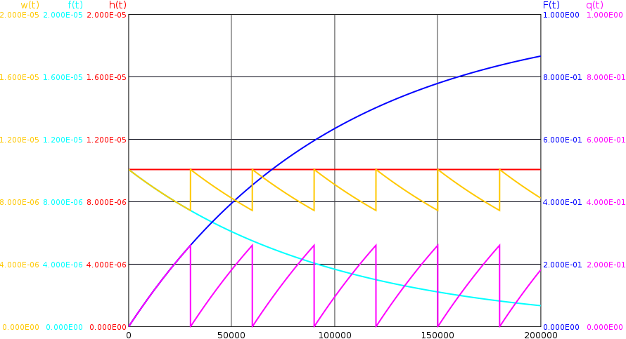
In contrast to the density \(f(t)\) \(w(t)\) never becomes zero, because due to the repair the system is always in a state (again), in which it can fail (again). Immediately after (complete) tests, i. e. when the unavailability returns to zero, the failure frequency increases again to the failure rate \(h(t)\). The integral of the failure frequency \(w(t)\) over time can thus become arbitrarily large. Only up to the first failure or the first test \(w(t)\) and \(f(t)\) are identical.
The failure rate, i. e. the frequency of transition to the failure state under the condition, that the system is capable of failure at time \(t\), is now calculated as
\(\seteqnumber{0}{}{49}\)\begin{equation} h(t) = \frac {w(t)}{A(t)} = \frac {w(t)}{1-Q(t)} \end{equation}
where \(A(t)\) denotes availability or \(Q(t)\) denotes unavailability at time \(t\).