Calculations for Functional Safety
Quantities, Formulas and Methods
5 Unavailability of complex functions
Unavailability is the essential parameter for safety functions, which are only rarely required. Examples of simple components that perform such safety functions are circuit breakers (should trip in case of overcurrent), pressure relief valves (should open in case of overpressure) or ceiling sprinklers (should release water in case of excessive temperature). Their functional architecture is shown in figure 11.
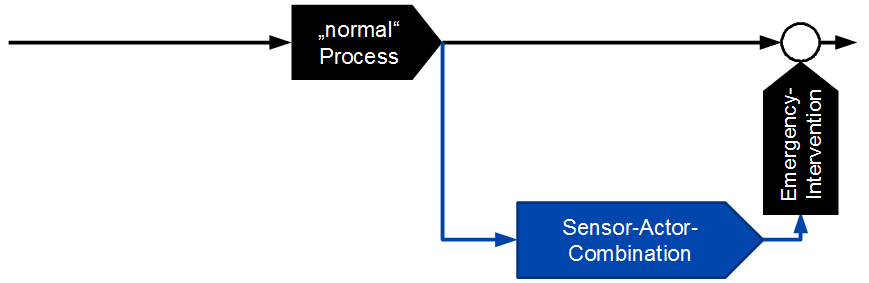
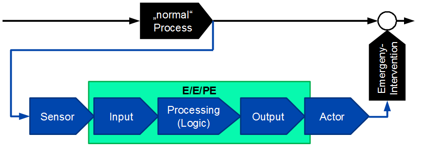
Of course, there are also more complex systems that perform infrequently needed safety functions, nowadays mostly computer-controlled. Examples are monitoring and emergency systems in the chemical industry or in power plants, fire detection and fire fighting systems, smoke extraction systems, evacuation systems, etc. Their architecture is exemplified in Figure 12. The term "process " is very broad in this context, it can be simply the normal operation of a building, apparatus or machine.
Normally, the existence of the safety function(s) is not noticed. Only in the case of a request (if this ever occurs) does it become apparent, whether the safety function is actually available 4. A safety-critical fault (i. e. one that prevents the safety function in the case of a request) can only be detected if the component or the system is tested regularly 5 or if it does not function when required.
The unavailability is practically always a time-dependent function \(Q(t)\). If there are no events with constant unavailability, the unavailability of a system \(Q_{\mathrm {sys}}\) at time \(t=0\) is zero. Only if there are events with constant unavailability, \(Q_{\mathrm {sys}}\) will be greater than zero already at \(t=0\). In any system there will be components, which have at least one failure mode which is not immediately apparent. The unavailability will therefore increase monotonically until the next test, and decrease to a smaller value (in the case of complete tests, to the value at \(t=0\)) immediately after a test. If there are failures that are never detected, the unavailability will increase, at least on average, until the end of the system’s operation.
Since it is never known at which point in time the safety function will be required, only the average value of the unavailability over the lifetime of the process or the safety system is of interest:
\(\seteqnumber{0}{}{50}\)\begin{equation} \label {eq:q_mean_} \overline {Q}=\frac {1}{T_{\mathrm {Life}}}\int \limits _0^{T_{\mathrm {Life}}} Q(t) dt \end{equation}
In [IEC 61508], this mean \(\overline {Q}\) is referred to as Probability of Failure on Demand (PFD for short).
4 Under certain circumstances, it also only becomes apparent then, whether the safety function is correctly designed, e. g. the actuators are correctly dimensioned, but this is not the subject of functional safety
5 for certain components a visual inspection may be sufficient
5.1 Calculation with fault trees
Frequently, the safety system is modeled with the help of fault trees. These are very suitable for modeling such systems, and the unavailability of the system \(\overline {Q_{\mathrm {sys}}}\) can be be computed very easily and mathematically accurately (assuming, of course, that the unavailabilities of the components are known).
Although ultimately only the mean value of the unavailability is of interest, nevertheless, according to formula (51), the time-dependent function must be calculated at a sufficient number of grid points and integrated over them.
The base events of a fault tree model the components with their failure modes and, if applicable, the measures for restoration. The standard model for a basic event is the so-called "restorable event", also referred to as a testable or repairable event, see appendix A.1. This model describes a (constant) failure rate and a (mean) detection time, as well as repair time, if applicable. If the failure is not detected by diagnostics or testing, i. e. remains in the system until the end of the operating time, the event shall be detected with the model "non-repairable event" according to Annex A.2 shall be described. In this case, non-constant failure rates are also possible. Sometimes the unavailability in case of the request also depends neither on a time since a last test nor on the age of the system, or the event does not describe a failure at all but rather the probability of the presence of an external boundary condition or the probability of an operator error. Then the unavailability is a constant (Appendix A.3).
As logical connections almost exclusively AND and OR are used, therefore only these shall be considered here. 6
Even if today the calculation is performed based on Binary Decision Diagrams (Binary Decision Diagrams, BDD for short), the calculation shall be explained here with the help of Minimal Cut-Sets (MCS).
A minimum cut is a combination of basic events, which is necessary and sufficient for the occurrence of the top event (for example, the failure of a safety function). For so-called coherent fault trees – which are fault trees that do not contain negating gates such as NOT, XOR, NAND, etc. – there is exactly one set of minimal cuts. For incoherent fault trees, we speak of prime implicants instead of minimal cuts, and there are in general several possible sets of prime implicants. Since negating gates rarely needed, they are not mentioned in the following.
6 So-called majority deciders (M-out-N) are nothing else than an abbreviation for an OR gate over several AND gates, so these are included. See section 6.1.6.
5.1.1 Unavailability of an AND operation
An AND operation of two or more basic events leads to a minimum cut with just these basic events. An AND-connection of branches of a tree usually leads to longer minimal cuts as well, the exact number and length depends on the structure of the linked branches.
The probability that a minimum cut is satisfied at a time \(t\), i. e., the unavailability resulting from a minimum cut, is
\(\seteqnumber{0}{}{51}\)\begin{equation} Q_{\mathrm {MCS}}(t)=\prod \limits _{j=1}^m Q_j(t) \label {eq:q_MCS} \end{equation}
Where \(m\) is the number of basic events in that minimal cut. The number \(m\) is called the order of the minimal cut.
-
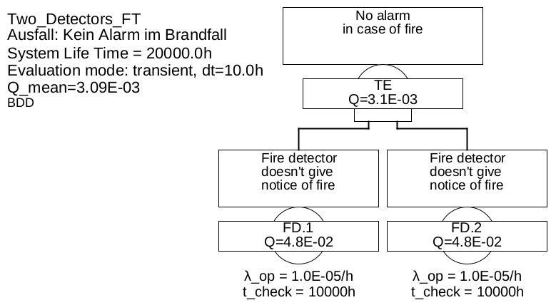
Example 5.1 There are two fire detectors in a room. Each has a failure rate of \(\lambda =\SI {1e-5}{\per \hour }\). The two fire detectors are tested simultaneously approximately every \(\SI {10000}{\hour }\) and replaced immediately in case a failure is detected in the test. What is the probability that none of them will report the fire in the event of a fire?
Figure 13 shows the corresponding fault tree. It consists of two base events of type "repairable event", which are linked by an AND gate.
There is only one minimal cut, namely {BM.1 & BM.2}. Since it contains two elements (literals), it is a minimal cut of second order. Consequently, using formulas (52) for the unavailability of the minimal cut and (39) for the unavailabilities of the fire detectors, the following applies
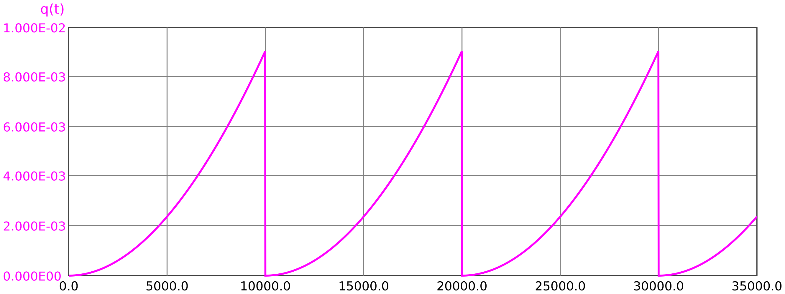
\(\seteqnumber{0}{}{52}\)\begin{equation*} Q_{\mathrm {sys}}(t) = Q_{\mathrm {BM.1}}(t) \cdot Q_{\mathrm {BM.2}}(t) = Q_{\mathrm {BM}}^2(t) = \left ( 1-\mathrm {e}^{-\lambda (t \bmod T_{\mathrm {test}})} \right )^2 = 1 - 2\mathrm {e}^{-\lambda (t \bmod T_{\mathrm {test}})} + \mathrm {e}^{-2 \lambda (t \bmod T_{\mathrm {test}})} \end{equation*}
With the above quantities, a periodicity with a period of \(\SI {10 000}{\hour }\) is obtained, the exact progression is shown in figure 14.
Due to the periodicity it is sufficient to calculate the average value over one period:
\(\seteqnumber{0}{}{52}\)\begin{align*} \begin{split} \overline {Q}&=\frac {1}{T_{\mathrm {Life}}}\int \limits _0^{T_{\mathrm {Life}}} Q(t)\,dt =\frac {1}{\SI {10000}{\hour }} \int \limits _{\SI {0}{\hour }}^{\SI {10000}{\hour }} 1 - 2\mathrm {e}^{-\lambda t} + \mathrm {e}^{-2 \lambda t}\,dt \\ &=\frac {1}{\SI {10000}{\hour }} \left [ t+\dfrac {2\mathrm {e}^{-\lambda t}}{\lambda } - \dfrac {\mathrm {e}^{-2\lambda t}}{2\lambda } \right ]_{\SI {0}{\hour }}^{\SI {10000}{\hour }} =\num {0.00309459}... \approx \num {3.1e-3} \end {split} \end{align*} The system usage time (lifetime) does not matter because of the periodic tests.
The reader may determine by his own calculation, that using the simplified formula \(Q_{\mathrm {BM}}(t)\lessapprox \lambda \cdot t\) instead of the exact formula used here \(Q_{\mathrm {BM}}(t)=1-\exp (-\lambda t)\) practically the same result is calculated.
5.1.2 Unvailability of an OR operation
An OR-operation of two or more basic events leads to a corresponding number of minimal cuts. An OR-operation of branches of a tree usually also leads to several minimal cuts, the exact number depends on the structure of the linked branches.
The total unavailability of the system is approximately the sum of the unavailabilities of the \(n\) minimal cuts:
\(\seteqnumber{0}{}{52}\)\begin{equation} Q_{\mathrm {sys}}(t) \lessapprox \sum \limits _{i=1}^{n_{\mathrm {MCS}}} Q_{\mathrm {MCS},i}(t) = \sum \limits _{i=1}^{n_{\mathrm {MCS}}} \left ( \prod \limits _{j=1}^{m_{\mathrm {Lit},i}} Q_j(t) \right ) \label {eq:q_sys_approx} \end{equation}
This formula is an approximation that only holds, when the individual unavailabilities are very small.
A better approximation, which can be calculated almost as easily, is the Esary-Proschan formula:
\(\seteqnumber{0}{}{53}\)\begin{equation} Q_{\mathrm {sys}}(t) \lessapprox 1-\prod \limits _{i=1}^{n_{\mathrm {MCS}}} \left ( 1-Q_{\mathrm {MCS},i}(t) \right ) \label {eq:q_sys_esary_proschan} \end{equation}
This approximation can be used well in practice, since it is always conservative (i. e. \(Q_{\mathrm {sys}}(t)\) never estimates too small), tends towards the exact result for small unavailabilities, and does not become larger than one for large unavailabilities. 7
The exact result is obtained by disjoint decomposition of the minimum cuts. A method for disjoint decomposition is described in [EN 61025]. However, this is only suitable for very small fault trees 8.
Binary decision diagrams (BDDs) can be created with little effort even for very large fault trees, without having to determine minimum cuts at all. Moreover, they already imply disjunction in the calculation. Therefore, they allow an exact calculation of the unavailability with much less effort than the approximation via minimal cuts. Finally, BDDs are by far the fastest method for determining the minimum cuts. Modern FTA tools therefore use BDDs for all operations.
7 one can also estimate a lower bound via minimal paths, but this differs so much from the actual value in practical tasks that it is meaningless
8 and for these the overlap of the minimum cuts is small anyway for correctly designed systems, a disjoint decomposition is unnecessary
-
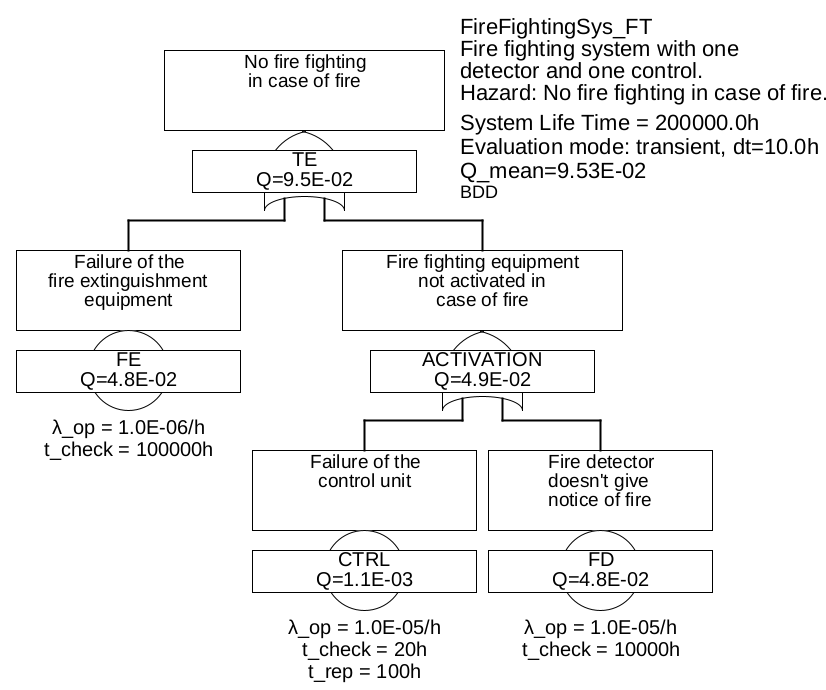
Example 5.2 In principle, an automatic fire extinguishing system consists of a fire detector (FD), a control unit (CTRL) and an fire extinguishing unit (FE). A fire is extinguished only if these three units function in the event of a fire.
This is modeled by the fault tree shown in Figure 15. Mathematically, one could place all three basic events directly under the upper OR gate, but this would violate the FTA rule "top-down design". This rule states that a fault tree shall always be developed from the top event down, and is one of the most important rules of all. And if you think about why the extinguishing system does not extinguish, it can only be because it itself is not working or that it is not activated. The control system and fire detectors only come into play when it comes to the question of why the extinguishing system is not activated, i. e. one level lower.
There are three minimal cuts, namely {FE}, {CTRL} and {FD}. All three are first order. If one uses the approximate formula (53) for the system nonavailability, one obtains
\(\seteqnumber{0}{}{54}\)\begin{equation*} Q_{\mathrm {sys}}(t) \lessapprox Q_{\mathrm {FE}}(t) + Q_{\mathrm {CTRL}}(t) + Q_{\mathrm {FD}}(t) \end{equation*}
and thus for the mean value
\(\seteqnumber{0}{}{54}\)\begin{equation*} \overline {Q_{\mathrm {sys}}} \lessapprox \overline {Q_{\mathrm {FE}}} + \overline {Q_{\mathrm {CTRL}}} + \overline {Q_{\mathrm {FD}}} \end{equation*}
Using the values mentioned in figure 15 and the approximation formulas (41) and (47), we finally obtain
\(\seteqnumber{0}{}{54}\)\begin{align*} \begin{split} \overline {Q_{\mathrm {sys}}} &\approx \num {0.5} \lambda _{\mathrm {FE}} T_{\mathrm {Test,FE}} + \lambda _{\mathrm {CTRL}} ( \num {0.5}\,T_{\mathrm {Test,CTRL}} + T_{\mathrm {MRT,CTRL}} ) + \num {0.5} \lambda _{\mathrm {FD}} T_{\mathrm {Test,FD}}\\ &= \num {0.05} + \num {0.0011} + \num {0.05} = \num {0.1011} \end {split} \end{align*} This approximate calculation differs from the exact value (not derived here) \(Q=\num {0.0953}...\) by only 5% — an accuracy absolutely sufficient for practice.
If one uses the estimation according to Esary-Proschan (54), one obtains
\(\seteqnumber{0}{}{54}\)\begin{equation*} Q_{\mathrm {sys}}(t) \lessapprox 1-\left [ ( 1-Q_{\mathrm {FE}}(t) ) \cdot ( 1-Q_{\mathrm {CTRL}}(t) ) \cdot ( 1-Q_{\mathrm {FD}}(t) ) \right ] \end{equation*}
Using the same approximations as before for the individual unavailabilities, we obtain for the mean system unavailability
\(\seteqnumber{0}{}{54}\)\begin{align*} \begin{split} \overline {Q_{\mathrm {sys}}} &\lessapprox 1-\big [ ( 1-\num {0.5} \lambda _{\mathrm {FE}} T_{\mathrm {Test,FE}} ) \\ &\qquad \quad \cdot ( 1-\lambda _{\mathrm {CTRL}} ( \num {0.5}\,T_{\mathrm {Test,CTRL}} + T_{\mathrm {MRT,CTRL}} ) ) \cdot ( 1- \num {0.5} \lambda _{\mathrm {FD}} T_{\mathrm {Test,FD}} ) \big ] \\ &=1-\left [(1-\num {0.05})\cdot (1-\num {0.0011})\cdot (1-\num {0.05})\right ]=\num {0.09849}... \end {split} \end{align*} This approximation differs from the exact value \(Q=\num {0.0953}...\) by only 3%.
5.1.3 Unavailability of combinations of AND and OR gates
For such simple systems as in the previous examples, one will hardly use fault tree. Practically, fault trees always consist of a plurality of AND and OR gates, which often link a multitude of basic events.
-
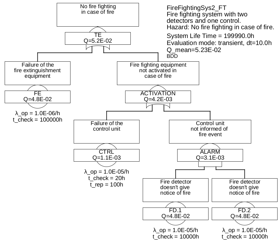
Example 5.3 Finally, the two previous examples are to be combined. Let the two smoke detectors be redundant again, i. e. mounted next to each other and interconnected in such a way, that one of them is sufficient to report a fire.
The fault tree is shown in Figure 16.
The three minimum cuts are: {FE}, {CTRL}, {FD.1 & FD.2}
According to approximate formula (53), system unavailability is approximately:
\(\seteqnumber{0}{}{54}\)\begin{equation*} Q_{\mathrm {sys}}(t) \lessapprox \sum \limits _{j=1}^n Q_{\mathrm {MCS},i}(t) = Q_{\mathrm {FE}}(t) + Q_{\mathrm {CTRL}}(t) + Q_{\mathrm {FD.1}}(t) \cdot Q_{\mathrm {FD.2}}(t) \end{equation*}
For the interested reader who is familiar with BDDs, the BDD should still be given for the sake of completeness.
If you select the variable order Extinguishing device (FE), Control (CTRL), Fire detector.1 (FD.1), Fire detector.2 (FD.2), the binary decision diagram BDD shown in Figure 17 is obtained.
An exact formula for system unavailability can be derived directly from the BDD:
\(\seteqnumber{0}{}{54}\)\begin{equation*} Q_{\mathrm {sys}}(t) = Q_{\mathrm {FE}}(t) + (1-Q_{\mathrm {FE}}(t)) \cdot \left [ Q_{\mathrm {CTRL}}(t) + (1-Q_{\mathrm {CTRL}}(t)) \cdot \left ( Q_{\mathrm {FD.1}}(t) \cdot Q_{\mathrm {FD.2}}(t) \right ) \right ] \end{equation*}
In this formula, all events are automatically disjoint. It should be noted that other formulas result with other variable orders, these are however all mathematically equivalent.

If we compare the exact formula with the approximation formula in the last example, we see immediately, that for all fault trees which do not contain negating gates the approximate formula (53) always gives a too large result. For small fault trees, the difference is negligible for all correctly designed systems 9, however, for large fault trees with many thousands of minimum cuts, even then the error can become very large. Therefore, large fault trees can practically only be calculated with BDDs, especially since already the determination of minimum cuts is practically only possible with the help of BDDs for large fault trees (even better with ternary decision diagrams).
9 correct design means that the test intervals are appropriate to the failure rates, so that all unavailabilities are very small at all times
5.1.4 Transient and steady-state computation, computing with averages
In general, to determine the average unavailability of a system, the integral must be calculated according to formula (51), as shown in example 5.1. Practically this means that the fault tree must be calculated for many time points, which can take some time for large fault trees even with modern computers. Here, of course, a possibly existing periodicity can be exploited, as also happened in example 5.1. If there is no periodicity (for example because there is at least one event without regular tests), then there will be no quasi-stationary state 10 set. In this case, the calculation must always be performed according to formula (51), i. e. numerical integration over the lifetime. Since this calculation considers also transient, i. e. non-periodic processes correctly, it is called transient calculation, in [ASTRA TM] simply time-dependent calculation.
To reduce the computation time, one can come up with the idea, to calculate the fault tree only once with the mean values of the unavailabilities of the basic events. This calculation assumes a steady-state quasi-stationary condition, and is therefore also called stationary calculation.
However, the calculation with mean values is not correct even in the steady state, because this would swap integral and product in the order, which is mathematically wrong:
\(\seteqnumber{0}{}{54}\)\begin{equation*} \overline {Q_{\mathrm {MCS}}} = \frac {1}{T_{\mathrm {Life}}}\int \limits _0^{T_{\mathrm {Life}}} Q(t)\,dt = \frac {1}{T_{\mathrm {Life}}}\int \limits _0^{T_{\mathrm {Life}}} \prod _{i=1}^n Q_i(t) \,dt \quad \neq \quad \prod _{i=1}^n \frac {1}{T_{\mathrm {Life}}} \int \limits _0^{T_{\mathrm {Life}}} Q_i(t) \,dt = \prod _{i=1}^n \overline {Q_i} \end{equation*}
The size of the error that occurs when calculating with mean values, depends on many parameters. In the case of two similar AND-linked events as in example 5.1, which are tested at the same time, the calculated result is about 1/3 too small:
\(\seteqnumber{0}{}{54}\)\begin{equation*} \overline {Q_{\mathrm {FD.1}}} \cdot \overline {Q_{\mathrm {FD.2}}} \approx \num {4.8e-2} \cdot \num {4.8e-2} \approx \num {2.3e-3}... \neq \num {3.1e-3} \end{equation*}
The error 1/3 comes from the integration of the quadratic term, which is responsible for the parabolic sections clearly visible in figure 14. Formula-wise this becomes particularly clear, if one uses the approximate formula \(Q(t)\lessapprox \lambda \cdot t\):
\(\seteqnumber{0}{}{54}\)\begin{equation*} \overline {Q_{\mathrm {correkt}}} = \frac {1}{T}\int \limits _0^T Q_1(t) \cdot Q_2(t)\,dt \approx \frac {1}{T}\int \limits _0^T \lambda t \cdot \lambda t\,dt = \frac {\lambda ^2}{3T} T^3 = \frac {\lambda ^2 T^2}{3} \end{equation*}
\(\seteqnumber{0}{}{54}\)\begin{equation*} \overline {Q_{\mathrm {wrong}}} = \frac {1}{T}\int \limits _0^T Q_1(t)\,dt \cdot \frac {1}{T}\int \limits _0^T Q_2(t)\,dt \approx \left ( \frac {1}{T}\int \limits _0^T \lambda t\,dt \right )^2 = \left ( \frac {\lambda }{2T} T^2\right )^2 = \frac {\lambda ^2 T^2}{4} \end{equation*}
For higher powers, i. e. higher order minimum cuts, the relative error becomes even larger, however, their absolute contribution is usually only small. A calculation with mean values can therefore be used in practice for rough calculations, but the final calculation should always be done according to formula (51), which makes a numerical integration necessary.
It should be noted, that a stationary calculation can also be performed with maximum values instead of mean values. In this case, the calculated unavailability is always (quite) conservative.
10 quasi-stationary means, that the unavailability may fluctuate around a mean value, but the mean value does not change with time
5.2 Calculation with Markov Models
System unavailability can also be calculated using Markov models. Markov models represent the states in which a system can be, as well as the transitions between the states. In classical Markov models, transitions are described by means of transition rates. Transitions away from the original state, in particular failures, are usually abbreviated as \(\lambda \). Transitions toward the original state, i. e., measures of restoration, are usually abbreviated as \(\mu \). Thus, a Markov model is mathematically described by a linear differential equation system:
\(\seteqnumber{0}{}{54}\)\begin{equation} \dot {\vec {p}}(t) = A(t)\,\vec {p}(t) \end{equation}
Here \(A(t)\) is the (generally time-dependent) transition matrix and \(\vec {p}\) is the vector of the residence probabilities of the system states.
Since the system is in exactly one state at any time, the sum of all state probabilities must always be one:
\(\seteqnumber{0}{}{55}\)\begin{equation} \|\vec {p}(t)\| = \sum _{i=1}^n p_i(t) = 1 \end{equation}
The sum of the residence probabilities in the states \(p_j(t) \in \vec {p(t)}\), in which the safety function is not given, indicates the system unavailability:
\(\seteqnumber{0}{}{56}\)\begin{equation} \label {eq:mm_sum_unavail} Q(t) = \sum _{j=1}^m p_j(t) \end{equation}
The mean unavailability is again given by formula (51).
The restoration rate \(\mu \) is almost always defined in the literature as the reciprocal of the mean recovery time: 11
\(\seteqnumber{0}{}{57}\)\begin{equation} \label {eq:mu} \mu \stackrel {\mathrm {def}}{=} 1 / \mathrm {MTTR} \end{equation}
For errors that are detected by regular tests, this results in the following for the restoration rate
\(\seteqnumber{0}{}{58}\)\begin{equation} \label {eq:mu_latent} \mu = 1 / \mathrm {MTTR} = \frac {1}{\num {0.5}\cdot T_{\mathrm {test}}} = 2/T_{\mathrm {test}} \end{equation}
11 That this is in fact a definition and not a factually justifiable formula, becomes visible in example 5.4 with example 5.5
-
Example 5.4 Figure 18 shows the Markov model for fire detection using redunant fire detectors, as considered in Example 5.1.
The failure rates \(\lambda \) for the fire detectors are indicated above the transition arrows in each case, the recovery rates \(\mu \) below each and indicated with a small arrow for the opposite direction. 12.
With the state vector
\(\seteqnumber{0}{}{59}\)\begin{equation*} \vec {p}= \begin{pmatrix} \mathrm {OK}\\ \mathrm {FD.1}\\ \mathrm {FD.2}\\ \mathrm {FD.1+FD.2} \end {pmatrix} \end{equation*}
applies to the linear differential equation system
\(\seteqnumber{0}{}{59}\)\begin{equation} \label {eq:ldgs_red_bm} \begin{pmatrix} -2\lambda & \mu & \mu & 0\\ \lambda & -\mu -\!\lambda & 0 & \mu \\ \lambda & 0 & -\mu -\!\lambda & \mu \\ 0 & \lambda & \lambda & -2\mu \end {pmatrix} \,\vec {p}(t)=\dot {\vec {p}}(t) \end{equation}
5.2.1 Stationary calculation
If every failure is detectable, there will also be a transition out of each state. Consequently, the states will be in equilibrium after an arbitrarily long time, so the time derivative of the state vector will become zero. If all detection and repair times are relatively short in relation to the lifetime of the system, the equilibrium will be practically taken after relatively short time.
The residence probabilities in this stationary system state can be easily calculated, by setting \(\dot {\vec {p}}(t)=0\) and then replacing any equation by the sum of the state probabilities, which must always be one.
Since the steady state lasts forever, the transient has no significant effect on the integral in formula (51), so the mean value of the unavailability is approximately equal to the unavailability in the steady state:
\(\seteqnumber{0}{}{60}\)\begin{equation} \overline {Q_{\mathrm {sys}}} \approx Q_{\mathrm {stat}} \end{equation}
-
Example 5.5 Replacing the fourth row in equation system (60) with the sum row, then the stationary solution is described by the following linear equation system:
\(\seteqnumber{0}{}{61}\)\begin{equation*} \begin{pmatrix} -2\lambda & \mu & \mu & 0\\ \lambda & -\mu -\!\lambda & 0 & \mu \\ \lambda & 0 & -\mu -\!\lambda & \mu \\ 1 & 1 & 1 & 1 \end {pmatrix} \,\vec {p_{\mathrm {stat}}}= \begin{pmatrix} 0\\ 0\\ 0\\ 1 \end {pmatrix} \end{equation*}
For the state vector in the steady state we get
\(\seteqnumber{0}{}{61}\)\begin{equation*} \renewcommand *{\arraystretch }{1.8} \vec {p_{\mathrm {stat}}}= \begin{pmatrix} \mathrm {OK}\\ \mathrm {FD.1}\\ \mathrm {FD.2}\\ \mathrm {FD.1+FD.2} \end {pmatrix} = \begin{pmatrix} \dfrac {{{\mu }^{2}}}{{{\mu }^{2}}+2\lambda \mu +{{\lambda }^{2}}}\\ \dfrac {\lambda \mu }{{{\mu }^{2}}+2\lambda \mu +{{\lambda }^{2}}}\\ \dfrac {\lambda \mu }{{{\mu }^{2}}+2\lambda \mu +{{\lambda }^{2}}}\\ \dfrac {{{\lambda }^{2}}}{{{\mu }^{2}}+2\lambda \mu +{{\lambda }^{2}}} \end {pmatrix} \end{equation*}
The unavailability is the residence probability of the state FD.1+FD.2, also \(\overline {Q_{\mathrm {stat}}}=\dfrac {\lambda ^2}{\mu ^2+2\lambda \mu +\lambda ^2}\).
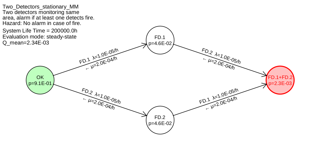
With the numerical values used for example 5.1 \(\lambda =\SI {1.0E-5}{\per \hour }\) and \(T_{\mathrm {test}}=\SI {10000}{\hour }\) we get \(\mu =2/(\SI {10000}{\hour })=\SI {2.0E-4}{\per \hour }\) and thus
\(\seteqnumber{0}{}{61}\)\begin{equation*} \overline {Q_{\mathrm {stat}}} =\dfrac {(\SI {1.0E-5}{\per \hour })^{2}} {(\SI {2.0E-4}{\per \hour })^2+2\cdot \SI {1.0E-5}{\per \hour }\cdot \SI {2.0E-4}{\per \hour }+(\SI {1.0E-5}{\per \hour })^2} \approx \num {0.0023} \end{equation*}
The mean unavailability in example 5.1 was exactly calculated to be \(\overline {Q_{\mathrm {sys}}}=\num {0.003094}...\), so the result obtained via the stationary evaluation of the Markov model is clearly too optimistic. On the one hand, this is due to the fact that formula (58) is only valid for continuous maintenance and repair, and formula (59) is always somewhat optimistic, but also because of the structure of the Markov model, which obviously does not reflect reality correctly — see the next example.
5.2.2 Transient calculation
In many practical applications, the steady state is not even approached, because the operating time is too short. If there are failures that cannot be detected or repaired, there are even absorbing states, so the steady state is given by the accumulation of the probability of residence in one or more failure states, so that \(Q(t \rightarrow \infty )=1\) holds 13. In this case, the stationary solution of the differential equation system is of no interest. Instead, the mean unavailability must be calculated by formula (51) during the transition from the original state to the end of the system’s operating time. This requires numerical integration of the differential equation system.
Numerical integration opens up possibilities for modeling that go beyond classical Markov models. In particular, it is possible to use time-varying transition rates and even to consider transitions at specific points in time. The latter in turn enables the realistic consideration of regular tests.
-
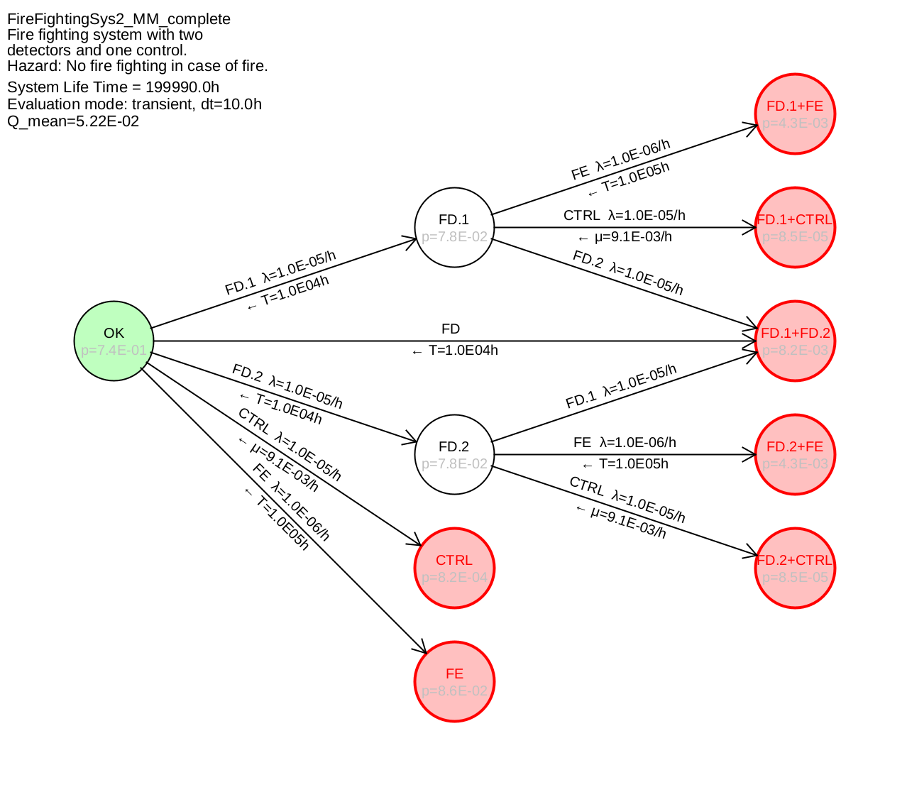
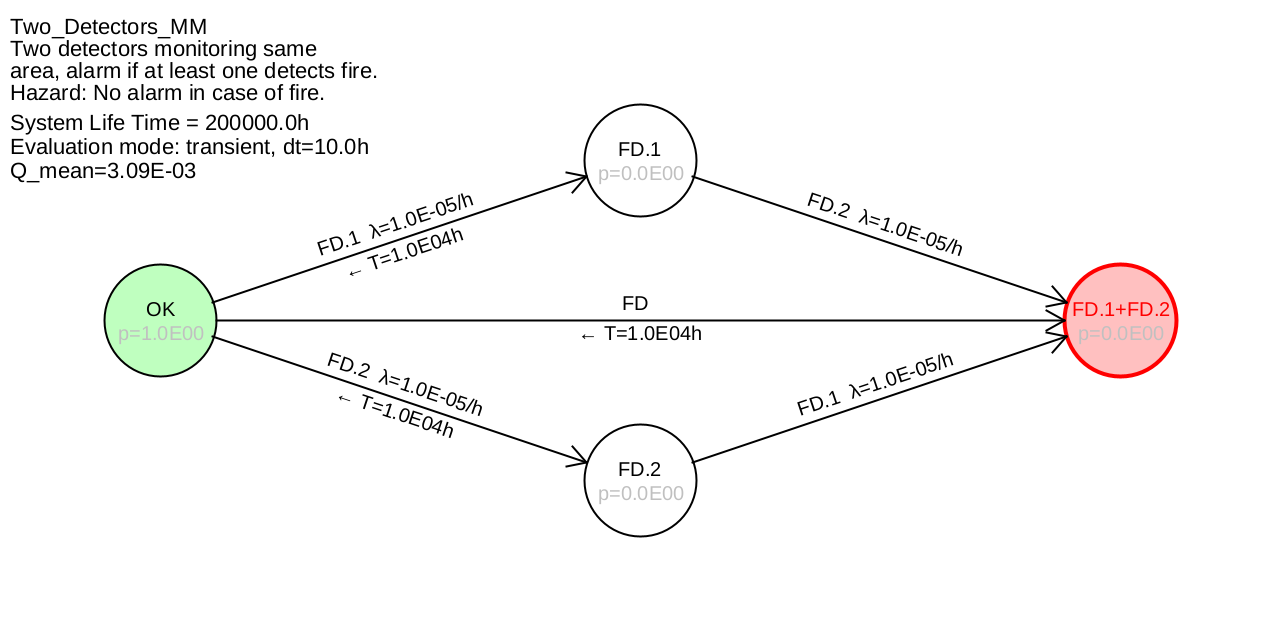
Example 5.6 Figure 19 shows a Markov model for the redundant fire detectors, in which it is taken into account that the tests, and thus the recovery, are not continuous, but occur at specific points in time. Furthermore, it is considered, that in case of defect of both fire detectors (state "FD.1+FD.2") both defects are detected at the same time and also the repair takes place at the same time, thus the system is restored to its original state.
Note: No failure rate is given at the transition arrow from "OK" to "FD.1+FD.2", therefore this is zero. Only the regular recovery every 10000 h is relevant here, this is under the transition arrow and is indicated with a small arrow to the left. Conversely, under the transition arrows "FD.1" and "FD.2" to "FD.1+FD.2" no restoration is stated, so this is zero.
The result of this modeling and calculation with an integration step size of 10 hours is \(Q=\num {3.09e-3}\) and now practically agrees with the exact value.
Classical Markov models with constant transition rates are only conditionally suitable for the calculation of unavailability, the results are usually too optimistic. Extended Markov models with discrete-time transitions allow realistic modeling and calculation and are therefore much more suitable.
It must be mentioned that the calculation of discrete-time transitions requires a sufficiently small integration step size. For small test intervals or even continuous diagnosis, constant transition rates must be used.
-
Example 5.7 Figure 20 shows the Markov model for the fire extinguishing system with redundant fire detectors introduced in Example 5.3. The recovery of the control CTRL is treated as a continuous transition, since the integration step size of 10 h is only slightly smaller than the test interval (20 h). The result is consistent with that of the fault tree.